Download to read offline


![Chapter 2 (Overview of Supervised Learning)
Statistical Decision Theory
We assume a linear model: that is we assume y = f(x) + ε, where ε is a random variable
with mean 0 and variance σ2
, and f(x) = xT
β. Our expected predicted error (EPE) under
the squared error loss is
EPE(β) =
Z
(y − xT
β)2
Pr(dx, dy) . (1)
We regard this expression as a function of β, a column vector of length p + 1. In order to
find the value of β for which it is minimized, we equate to zero the vector derivative with
respect to β. We have
∂EPE
∂β
=
Z
2 (y − xT
β) (−1)x Pr(dx, dy) = −2
Z
(y − xT
β)xPr(dx, dy) . (2)
Now this expression has two parts. The first has integrand yx and the second has integrand
(xT
β)x.
Before proceeding, we make a quick general remark about matrices. Suppose that A, B and
C are matrices of size 1 × p matrix, p × 1 and q × 1 respectively, where p and q are positive
integers. Then AB can be regarded as a scalar, and we have (AB)C = C(AB), each of these
expressions meaning that each component of C is multiplied by the scalar AB. If q > 1,
the expressions BC, A(BC) and ABC are meaningless, and we must avoid writing them.
On the other hand, CAB is meaningful as a product of three matrices, and the result is the
q × 1 matrix (AB)C = C(AB) = CAB. In our situation we obtain (xT
β)x = xxT
β.
From ∂EPE/∂β = 0 we deduce
E[yx] − E[xxT
β] = 0 (3)
for the particular value of β that minimizes the EPE. Since this value of β is a constant, it
can be taken out of the expectation to give
β = E[xxT
]−1
E[yx] , (4)
which gives Equation 2.16 in the book.
We now discuss some points around Equations 2.26 and 2.27. We have
β̂ = (XT
X)−1
XT
y = (XT
X)−1
XT
(Xβ + ε) = β + (XT
X)−1
XT
ε.
So
ŷ0 = xT
0 β̂ = xT
0 β + xT
0 (XT
X)−1
XT
ε. (5)
This immediately gives
ŷ0 = xT
0 β +
N
X
i=1
ℓi(x0)εi
3](https://image.slidesharecdn.com/asolutionmanualandnotesfortheelementsofstatisticallearning-230807171037-5c97f6ed/85/A-Solution-Manual-and-Notes-for-The-Elements-of-Statistical-Learning-pdf-3-320.jpg)
![This completes our discussion of Equations 2.27 and 2.28.
Notes on Local Methods in High Dimensions
The most common error metric used to compare different predictions of the true (but un-
known) mapping function value f(x0) is the mean square error (MSE). The unknown in the
above discussion is the specific function mapping function f(·) which can be obtained via
different methods many of which are discussed in the book. In supervised learning to help
with the construction of an appropriate prediction ŷ0 we have access to a set of “training
samples” that contains the notion of randomness in that these points are not under complete
control of the experimenter. One could ask the question as to how much square error at our
predicted input point x0 will have on average when we consider all possible training sets T .
We can compute, by inserting the “expected value of the predictor obtained over all training
sets”, ET (ŷ0) into the definition of quadratic (MSE) error as
MSE(x0) = ET [f(x0) − ŷ0]2
= ET [ŷ0 − ET (ŷ0) + ET (ŷ0) − f(x0)]2
= ET [(ŷ0 − ET (ŷ0))2
+ 2(ŷ0 − ET (ŷ0))(ET (ŷ0) − f(x0)) + (ET (ŷ0) − f(x0))2
]
= ET [(ŷ0 − ET (ŷ0))2
] + (ET (ŷ0) − f(x0))2
.
Where we have expanded the quadratic, distributed the expectation across all terms, and
noted that the middle term vanishes since it is equal to
ET [2(ŷ0 − ET (ŷ0))(ET (ŷ0) − f(x0))] = 0 ,
because ET (ŷ0) − ET (ŷ0) = 0. and we are left with
MSE(x0) = ET [(ŷ0 − ET (ŷ0))2
] + (ET (ŷ0) − f(x0))2
. (10)
The first term in the above expression ET [(ŷ0 −ET (ŷ0))2
] is the variance of our estimator ŷ0
and the second term (ET (ŷ0) − f(x0))2
is the bias (squared) of our estimator. This notion
of variance and bias with respect to our estimate ŷ0 is to be understood relative to possible
training sets, T , and the specific computational method used in computing the estimate ŷ0
given that training set.
Exercise Solutions
Ex. 2.1 (target coding)
The authors have suppressed the context here, making the question a little mysterious. For
example, why use the notation ȳ instead of simply y? We imagine that the background is
something like the following. We have some input data x. Some algorithm assigns to x the
probability yk that x is a member of the k-th class. This would explain why we are told to
assume that the sum of the yk is equal to one. (But, if that reason is valid, then we should
5](https://image.slidesharecdn.com/asolutionmanualandnotesfortheelementsofstatisticallearning-230807171037-5c97f6ed/85/A-Solution-Manual-and-Notes-for-The-Elements-of-Statistical-Learning-pdf-5-320.jpg)


![Ex. 2.7 (forms for linear regression and k-nearest neighbor regression)
To simplify this problem lets begin in the case of simple linear regression where there is only
one response y and one predictor x. Then the standard definitions of y and X state that
yT
= (y1, . . . , yn), and XT
=
1 · · · 1
x1 · · · xn
.
Part (a): Let’s first consider linear regression. We use (2.2) and (2.6), but we avoid just
copying the formulas blindly. We have β̂ = XT
X
−1
XT
y, and then set
ˆ
f(x0) = [x0 1]β̂ = [x0 1] XT
X
−1
XT
y.
In terms of the notation of the question,
ℓi(x0; X ) = [x0 1] XT
X
−1
1
xi
for each i with 1 ≤ i ≤ n.
More explicitly, XT
X =
n
P
xi
P
xi
P
x2
i
which has determinant (n−1)
P
i x2
i −2n
P
ij xixj.
This allows us to calculate XT
X
−1
and ℓi(x0; X ) even more explicitly if we really want to.
In the case of k-nearest neighbor regression ℓi(x0; X ) is equal to 1/k if xi is one of the nearest
k points and 0 otherwise.
Part (b): Here X is fixed, and Y varies. Also x0 and f(x0) are fixed. So
EY|X
f(x0) − ˆ
f(x0)
2
= f(x0)2
− 2.f(x0).EY|X
ˆ
f(x0)
+ EY|X
ˆ
f(x0)
2
=
f(x0) − EY|X
ˆ
f(x0)
2
+ EY|X
ˆ
f(x0)
2
−
EY|X
ˆ
f(x0)
2
= (bias)2
+ Var( ˆ
f(x0))
Part (c): The calculation goes the same way as in (b), except that both X and Y vary.
Once again x0 and f(x0) are constant.
EX,Y
f(x0) − ˆ
f(x0)
2
= f(x0)2
− 2.f(x0).EX,Y
ˆ
f(x0)
+ EX,Y
ˆ
f(x0)
2
=
f(x0) − EX,Y
ˆ
f(x0)
2
+ EX,Y
ˆ
f(x0)
2
−
EX,Y
ˆ
f(x0)
2
= (bias)2
+ Var( ˆ
f(x0))
The terms in (b) can be evaluated in terms of the ℓi(x0; X ) and the distribution of εi. We
10](https://image.slidesharecdn.com/asolutionmanualandnotesfortheelementsofstatisticallearning-230807171037-5c97f6ed/85/A-Solution-Manual-and-Notes-for-The-Elements-of-Statistical-Learning-pdf-10-320.jpg)


![Chapter 3 (Linear Methods for Regression)
Notes on the Text
Linear Regression Models and Least Squares
For this chapter, given the input vector x, the model of how our scalar output y is generated
will assumed to be y = f(x) + ε = xT
β + ε for some fixed vector β of p + 1 coefficients, and
ε a scalar random variable with mean 0 and variance σ2
. With a full data set obtained of N
input/output pairs (xi, yi) arranged in the vector variables X and y, the space in which we
work is RN
. This contains vectors like y = (y1, . . . , yN ), and each column of X. The least
squares estimate of β is given by the book’s Equation 3.6
β̂ = (XT
X)−1
XT
y . (13)
We fix X and compute the statistical properties of β̂ with respect to the distribution Y |X.
Using the fact that E(y) = Xβ, we obtain
E(β̂) = (XT
X)−1
XT
Xβ = β . (14)
Using Equation 14 for E(β̂) we get
β̂ − E(β̂) = (XT
X)−1
XT
y − (XT
X)−1
XT
Xβ
= (XT
X)−1
XT
(y − Xβ)
= (XT
X)−1
XT
ε,
where ε is a random column vector of dimension N. The variance of β̂ is computed as
Var[β̂] = E[(β̂ − E[β̂])(β̂ − E[β̂])T
]
= (XT
X)−1
XT
E (εε)T
X(XT
X)−1
= (XT
X)−1
XT
Var(ε)X(XT
X)−1
.
If we assume that the entries of y are uncorrelated and all have the same variance of σ2
(again given X), then Var[ε] = σ2
IN , where IN is the N × N identity matrix and the above
becomes
Var[β̂] = σ2
(XT
X)−1
XT
X(XT
X)−1
= (XT
X)−1
σ2
, (15)
which is Equation 3.8 in the book.
It remains to specify how to determine σ2
. To that end once β is estimated we can compute
σ̂2
=
1
N − p − 1
N
X
i=1
(yi − ŷi)2
=
1
N − p − 1
N
X
i=1
(yi − xT
i β)2
, (16)
and subsequently claim that this gives an unbiased estimate of σ2
. To see this, we argue as
follows.
14](https://image.slidesharecdn.com/asolutionmanualandnotesfortheelementsofstatisticallearning-230807171037-5c97f6ed/85/A-Solution-Manual-and-Notes-for-The-Elements-of-Statistical-Learning-pdf-14-320.jpg)

![See [1] and the accompanying notes for this text where the above expression is explicitly
derived from first principles. Alternatively one can follow the steps above. We can write the
denominator of the above expression for β1 as hx−x̄1, x−x̄1i. That this is true can be seen
by expanding this expression
hx − x̄1, x − x̄1i = xT
x − x̄(xT
1) − x̄(1T
x) + x̄2
n
= xT
x − nx̄2
− nx̄2
+ nx̄2
= xT
x −
1
n
(
X
xt)2
.
Which in matrix notation is given by
β̂1 =
hx − x̄1, yi
hx − x̄1, x − x̄1i
, (19)
or equation 3.26 in the book. Thus we see that obtaining an estimate of the second coefficient
β1 is really two one-dimensional regressions followed in succession. We first regress x onto
1 and obtain the residual z = x − x̄1. We next regress y onto this residual z. The direct
extension of these ideas results in Algorithm 3.1: Regression by Successive Orthogonalization
or Gram-Schmidt for multiple regression.
Another way to view Algorithm 3.1 is to take our design matrix X, form an orthogonal
basis by performing the Gram-Schmidt orthogonilization procedure (learned in introductory
linear algebra classes) on its column vectors, and ending with an orthogonal basis {zi}p
i=1.
Then using this basis linear regression can be done simply as in the univariate case by by
computing the inner products of y with zp as
β̂p =
hzp, yi
hzp, zpi
, (20)
which is the books equation 3.28. Then with these coefficients we can compute predictions
at a given value of x by first computing the coefficient of x in terms of the basis {zi}p
i=1 (as
zT
p x) and then evaluating
ˆ
f(x) =
p
X
i=0
β̂i(zT
i x) .
From Equation 20 we can derive the variance of β̂p that is stated in the book. We find
Var(β̂p) = Var
zT
p y
hzp, zpi
!
=
zT
p Var(y)zp
hzp, zpi2 =
zT
p (σ2
I)zp
hzp, zpi2
=
σ2
hzp, zpi
,
which is the books equation 3.29.
As stated earlier Algorithm 3.1 is known as the Gram-Schmidt procedure for multiple re-
gression and it has a nice matrix representation that can be useful for deriving results that
demonstrate the properties of linear regression. To demonstrate some of these, note that we
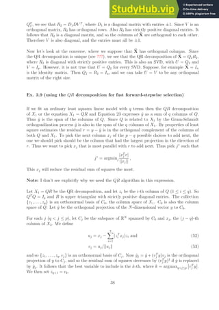
can write the Gram-Schmidt result in matrix form using the QR decomposition as
X = QR . (21)
19](https://image.slidesharecdn.com/asolutionmanualandnotesfortheelementsofstatisticallearning-230807171037-5c97f6ed/85/A-Solution-Manual-and-Notes-for-The-Elements-of-Statistical-Learning-pdf-19-320.jpg)
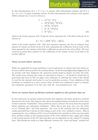
![0 2 4 6 8
0
20
40
60
80
100
Subset Size k
Residual
Sum−of−Squares
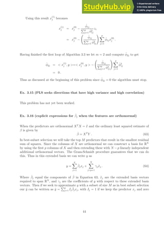
Figure 1: Duplication of the books Figure 3.5 using the code duplicate figure 3 5.R. This
plot matches quite well qualitatively and quantitatively the corresponding one presented in
the book.
I wanted to mention this point in case anyone reads the provided code for the all subsets
and ridge regression methods.
In duplicating the all-subsets and ridge regression results in this section we wrote our own R
code to perform the given calculations. For ridge regression an alternative approach would
have been to use the R function lm.ridge found in the MASS package. In duplicating the
lasso results in this section we use the R package glmnet [5], provided by the authors and
linked from the books web site. An interesting fact about the glmnet package is that for
the parameter settings α = 0 the elastic net penalization framework ignores the L1 (lasso)
penalty on β and the formulation becomes equivalent to an L2 (ridge) penalty on β. This
parameter setting would allow one to use the glmnet package to do ridge-regression if desired.
Finally, for the remaining two regression methods: principal component regression (PCR)
and partial least squares regression (PLSR) we have used the R package pls [7], which is a
package tailored to perform these two types of regressions.
As a guide to what R functions perform what coding to produce the above plots and table
21](https://image.slidesharecdn.com/asolutionmanualandnotesfortheelementsofstatisticallearning-230807171037-5c97f6ed/85/A-Solution-Manual-and-Notes-for-The-Elements-of-Statistical-Learning-pdf-21-320.jpg)
![we find
β̂ridge
= (XT
X + λI)−1
XT
y (28)
= (V D2
V T
+ λV V T
)−1
V DUT
y
= (V (D2
+ λI)V T
)−1
V DUT
y
= V (D2
+ λI)−1
DUT
y . (29)
Using this we can compute the product ŷridge
= Xβ̂ridge
. As in the above case for least
squares we find
ŷridge
= Xβ̂ridge
= UD(D2
+ λI)−1
DUT
y . (30)
Now note that in this last expression D(D2
+λI)−1
is a diagonal matrix with elements given
by
d2
j
d2
j +λ
and the vector UT
y is the coordinates of the vector y in the basis spanned by the
p-columns of U. Thus writing the expression given by Equation 30 by summing columns we
obtain
ŷridge
= Xβ̂ridge
=
p
X
j=1
uj
d2
j
d2
j + λ
uT
j y . (31)
Note that this result is similar to that found in Equation 27 derived for ordinary least squares
regression but in ridge-regression the inner products uT
j y are now scaled by the factors
d2
j
d2
j +λ
.
Notes on the effective degrees of freedom df(λ)
The definition of the effective degrees of freedom df(λ) in ridge regression is given by
df(λ) = tr[X(XT
X + λI)−1
XT
] . (32)
Using the results in the SVD derivation of the expression Xβ̂ridge
, namely Equation 30 but
without the y factor, we find the eigenvector/eigenvalue decomposition of the matrix inside
the trace operation above given by
X(XT
X + λI)−1
XT
= UD(D2
+ λI)−1
DUT
.
From this expression the eigenvalues of X(XT
X + λI)−1
XT
must be given by the elements
d2
j
d2
j +λ
. Since the trace of a matrix can be shown to equal the sum of its eigenvalues we have
that
df(λ) = tr[X(XT
X + λI)−1
XT
]
= tr[UD(D2
+ λI)−1
DUT
]
=
p
X
j=1
d2
j
d2
j + λ
, (33)
which is the books equation 3.50.
24](https://image.slidesharecdn.com/asolutionmanualandnotesfortheelementsofstatisticallearning-230807171037-5c97f6ed/85/A-Solution-Manual-and-Notes-for-The-Elements-of-Statistical-Learning-pdf-24-320.jpg)

![Below are just some notes scraped together over various emails discussing some facts that I
felt were worth proving/discussing/understanding better:
λ is allowed to range over (0, ∞) and all the solutions are different. But s is only allowed to
range over an interval (0, something finite). If s is increased further the constrained solution
is equal to the unconstrained solution. That’s why I object to them saying there is a one-to-
one correspondence. It’s really a one-to-one correspondence between the positive reals and
a finite interval of positive numbers.
I’m assuming by s above you mean the same thing the book does s = t/
Pp
1 | ˆ
βj|q
where q is
the ”power’ in the Lq regularization term. See the section 3.4.3 in the book) . Thus q = 1
for lasso and q = 2 for ridge. So basically as the unconstrained solution is the least squares
one as then all estimated betas approach the least square betas. In that case the largest
value for s is 1, so we actually know the value of the largest value of s. For values of s larger
than this we will obtain the least squares solution.
The one-to-one correspondence could be easily worked out by a computer program in any
specific case. I don’t believe there is a nice formula.
Notes on Least Angle Regression (LAR)
To derive a better connection between Algorithm 3.2 (a few steps of Least Angle Regression)
and the notation on the general LAR step “k” that is presented in this section that follows
this algorithm I found it helpful to perform the first few steps of this algorithm by hand and
explicitly writing out what each variable was. In this way we can move from the specific
notation to the more general expression.
• Standardize all predictors to have a zero mean and unit variance. Begin with all
regression coefficients at zero i.e. β1 = β2 = · · · = βp = 0. The first residual will be
r = y − ȳ, since with all βj = 0 and standardized predictors the constant coefficient
β0 = ȳ.
• Set k = 1 and begin start the k-th step. Since all values of βj are zero the first residual
is r1 = y − ȳ. Find the predictor xj that is most correlated with this residual r1. Then
as we begin this k = 1 step we have the active step given by A1 = {xj} and the active
coefficients given by βA1 = [0].
• Move βj from its initial value of 0 and in the direction
δ1 = (XT
A1
XA1 )−1
XT
A1
r1 =
xT
j r1
xT
j xj
= xT
j r1 .
Note that the term xT
j xj in the denominator is not present since xT
j xj = 1 as all
variables are normalized to have unit variance. The path taken by the elements in βA1
can be parametrized by
βA1 (α) ≡ βA1 + αδ1 = 0 + αxT
j r1 = (xT
j r1)α for 0 ≤ α ≤ 1 .
26](https://image.slidesharecdn.com/asolutionmanualandnotesfortheelementsofstatisticallearning-230807171037-5c97f6ed/85/A-Solution-Manual-and-Notes-for-The-Elements-of-Statistical-Learning-pdf-26-320.jpg)
![• Standardize the predictor variables xi for i = 1, 2, . . . , p to have mean zero and variance
one. Demean the response y.
• Given the design matrix X compute the product XT
X.
• Compute the eigendecomposition of XT
X as
XT
X = V D2
V T
.
The columns of V are denoted vm and the diagonal elements of D are denoted dm.
• Compute the vectors zm defined as zm = Xvm for m = 1, 2, . . . , p.
• Using these vectors zm compute the regression coefficients θ̂m given by
θ̂m =
zm, y
zm, zm
.
Note that we don’t need to explicitly compute the inner product zm, zm for each
m directly since using the eigendecomposition XT
X = V D2
V T
computed above this
is equal to
zT
mzm = vT
mXT
Xvm = vT
mV D2
V T
vm = (V T
vm)T
D2
(V T
vm) = eT
mD2
em = d2
m ,
where em is a vector of all zeros with a one in the mth spot.
• Given a value of M for 0 ≤ M ≤ p, the values of θ̂m, and zm the PCR estimate of y is
given by
ŷpcr
(M) = ȳ1 +
M
X
m=1
θ̂mzm .
While the value of β̂pcr
(M) which can be used for future predictions is given by
β̂pcr
(M) =
M
X
m=1
θ̂mvm .
This algorithm is implemented in the R function pcr wwx.R, and cross validation using this
method is implemented in the function cv pcr wwx.R. A driver program that duplicates the
results from dup OSE PCR N PLSR.R is implemented in pcr wwx run.R. This version of the
PCR algorithm was written to ease transformation from R to a more traditional programming
language like C++.
Note that the R package pcr [7] will implement this linear method and maybe more suitable
for general use since it allows input via R formula objects and has significantly more options.
29](https://image.slidesharecdn.com/asolutionmanualandnotesfortheelementsofstatisticallearning-230807171037-5c97f6ed/85/A-Solution-Manual-and-Notes-for-The-Elements-of-Statistical-Learning-pdf-29-320.jpg)
![We have seen that, for i 6= j, uj/vjj is orthogonal to xi, and the coefficient of xj in uj/vjj is
1. Permuting the columns of X so that the j-th column comes last, we see that uj/vjj = zj
(see Algorithm 3.1). By Equation 40,
kujk2
= uT
j uj =
p+1
X
r=1
vrjxT
r uj =
p+1
X
r=1
vrjδrj = vjj.
Then
kzjk2
=
kujk2
v2
jj
= vjj/v2
jj =
1
vjj
. (41)
Now zj/kzjk is a unit vector orthogonal to x1, . . . , xj−1, xj+1, . . . , xp+1. So
RSSj − RSS1 = hy, zj/kzjki2
=
hy, zji
hzj, zji
2
kzjk2
= β̂2
j /vjj,
where the final equality follows from Equation 41 and the book’s Equation 3.28.
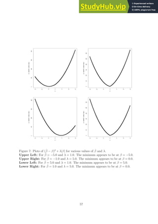
Ex. 3.2 (confidence intervals on a cubic equation)
In this exercise, we fix a value for the column vector β = (β0, β1, β2, β3)T
and examine
random deviations from the curve
y = β0 + β1x + β2x2
+ β3x3
.
For a given value of x, the value of y is randomized by adding a normally distributed variable
with mean 0 and variance 1. For each x, we have a row vector x = (1, x, x2
, x3
). We fix N
values of x. (In Figure 6 we have taken 40 values, evenly spaced over the chosen domain
[−2, 2].) We arrange the corresponding values of x in an N × 4-matrix, which we call X, as
in the text. Also we denote by y the corresponding N × 1 column vector, with independent
entries. The standard least squares estimate of β is given by β̂ = XT
X
−1
XT
y. We now
compute a 95% confidence region around this cubic in two different ways.
In the first method, we find, for each x, a 95% confidence interval for the one-dimensional
random variable u = x.β̂. Now y is a normally distributed random variable, and therefore
so is β̂ = (XT
X)−1
XT
y. Therefore, using the linearity of E,
Var(u) = E
xβ̂β̂T
xT
− E
xβ̂
.E
β̂T
xT
= xVar(β̂)xT
= x XT
X
−1
xT
.
This is the variance of a normally distributed one-dimensional variable, centered at x.β, and
the 95% confidence interval can be calculated as usual as 1.96 times the square root of the
variance.
32](https://image.slidesharecdn.com/asolutionmanualandnotesfortheelementsofstatisticallearning-230807171037-5c97f6ed/85/A-Solution-Manual-and-Notes-for-The-Elements-of-Statistical-Learning-pdf-32-320.jpg)
![In the second method, β̂ is a 4-dimensional normally distributed variable, centered at β, with
4 × 4 variance matrix XT
X
−1
. We need to take a 95% confidence region in 4-dimensional
space. We will sample points β̂ from the boundary of this confidence region, and, for each
such sample, we draw the corresponding cubic in green in Figure 6 on page 56. To see what
to do, take the Cholesky decomposition UT
U = XT
X, where U is upper triangular. Then
(UT
)−1
XT
X
U−1
= I4, where I4 is the 4×4-identity matrix. Uβ̂ is a normally distributed
4-dimensional variable, centered at Uβ, with variance matrix
Var(Uβ̂) = E
Uβ̂β̂T
UT
− E
Uβ̂
.E
β̂T
UT
= U XT
X
−1
UT
= I4
It is convenient to define the random variable γ = β̂ − β ∈ R4
, so that Uγ is a standard
normally distributed 4-dimensional variable, centered at 0.
Using the R function qchisq, we find r2
, such that the ball B centered at 0 in R4
of radius
r has χ2
4-mass equal to 0.95, and let ∂B be the boundary of this ball. Now Uγ ∈ ∂B if and
only if its euclidean length squared is equal to r2
. This means
r2
= kUγk2
= γT
UT
Uγ = γT
XT
Xβ.
Given an arbitrary point α ∈ R4
, we obtain β̂ in the boundary of the confidence region by
first dividing by the square root of γT
XT
Xγ and then adding the result to β.
Note that the Cholesky decomposition was used only for the theory, not for the purposes of
calculation. The theory could equally well have been proved using the fact that every real
positive definite matrix has a real positive definite square root.
Our results for one particular value of β are shown in Figure 6 on page 56.
Ex. 3.3 (the Gauss-Markov theorem)
(a) Let b be a column vector of length N, and let E(bT
y) = αT
β. Here b is fixed, and the
equality is supposed true for all values of β. A further assumption is that X is not random.
Since E(bT
y) = bT
Xβ, we have bT
X = αT
. We have
Var(αT
β̂) = αT
(XT
X)−1
α = bT
X(XT
X)−1
XT
b,
and Var(bT
y) = bT
b. So we need to prove X(XT
X)−1
XT
IN .
To see this, write X = QR where Q has orthonormal columns and is N × p, and R is p × p
upper triangular with strictly positive entries on the diagonal. Then XT
X = RT
QT
QR =
RT
R. Therefore X(XT
X)−1
XT
= QR(RT
R)−1
RT
QT
= QQT
. Let [QQ1] be an orthogonal
N × N matrix. Therefore
IN =
Q Q1
.
QT
QT
1
= QQT
+ Q1QT
1 .
Since Q1QT
1 is positive semidefinite, the result follows.
33](https://image.slidesharecdn.com/asolutionmanualandnotesfortheelementsofstatisticallearning-230807171037-5c97f6ed/85/A-Solution-Manual-and-Notes-for-The-Elements-of-Statistical-Learning-pdf-33-320.jpg)

![From this we see that by defining “centered” values of β as
βc
0 = β0 +
p
X
j=1
x̄jβj
βc
j = βi i = 1, 2, . . . , p ,
that the above can be recast as
N
X
i=1
yi − βc
0 −
p
X
j=1
(xij − x̄j)βc
j
!2
+ λ
p
X
j=1
βc
j
2
The equivalence of the minimization results from the fact that if βi minimize its respective
functional the βc
i ’s will do the same.
A heuristic understanding of this procedure can be obtained by recognizing that by shifting
the xi’s to have zero mean we have translated all points to the origin. As such only the
“intercept” of the data or β0 is modified the “slope’s” or βc
j for i = 1, 2, . . . , p are not
modified.
We compute the value of βc
0 in the above expression by setting the derivative with respect
to this variable equal to zero (a consequence of the expression being at a minimum). We
obtain
N
X
i=1
yi − βc
0 −
p
X
j=1
(xij − x̄j) βj
!
= 0,
which implies βc
0 = ȳ, the average of the yi. The same argument above can be used to
show that the minimization required for the lasso can be written in the same way (with βc
j
2
replaced by |βc
j |). The intercept in the centered case continues to be ȳ.
WWX: This is as far as I have proofed
Ex. 3.6 (the ridge regression estimate)
Note: I used the notion in original problem in [6] that has τ2
rather than τ as the variance
of the prior. Now from Bayes’ rule we have
p(β|D) ∝ p(D|β)p(β) (44)
= N (y − Xβ, σ2
I)N (0, τ2
I) (45)
Now from this expression we calculate
log(p(β|D)) = log(p(D|β)) + log(p(β)) (46)
= C −
1
2
(y − Xβ)T
(y − Xβ)
σ2
−
1
2
βT
β
τ2
(47)
35](https://image.slidesharecdn.com/asolutionmanualandnotesfortheelementsofstatisticallearning-230807171037-5c97f6ed/85/A-Solution-Manual-and-Notes-for-The-Elements-of-Statistical-Learning-pdf-35-320.jpg)
![here the constant C is independent of β. The mode and the mean of this distribution (with
respect to β) is the argument that maximizes this expression and is given by
β̂ = ArgMin(−2σ2
log(p(β|D)) = ArgMin((y − Xβ)T
(y − Xβ) +
σ2
τ2
βT
β) (48)
Since this is the equivalent to Equation 3.43 page 60 in [6] with the substitution λ = σ2
τ2 we
have the requested equivalence.
Exs3.6 and 3.7 These two questions are almost the same; unfortunately they are both
somewhat wrong, and in more than one way. This also means that the second-last paragraph
on page 64 and the second paragraph on page 611 are both wrong. The main problem is that
β0 is does not appear in the penalty term of the ridge expression, but it does appear in the
prior for β. . In Exercise 3.6, β has variance denoted by τ, whereas the variance is denoted
by τ2
in Exercise 3.7. We will use τ2
throughout, which is also the usage on page 64.
With X = (x1, . . . , xp) fixed, Bayes’ Law states that p(y|β).p(β) = p(β|y).p(y). So, the
posterior probability satisfies
p(β|y) ∝ p(y|β).p(β),
where p denotes the pdf and where the constant of proportionality does not involve β. We
have
p(β) = C1 exp −
kβk2
2τ2
!
and
p(y|β) = C2 exp −
ky − Xβk2
2σ2
!
for appropriate constants C1 and C2. It follows that, for a suitable constant C3,
p(β|y) = C3 exp −
ky − Xβk2
+ (σ2
/τ2
).kβk2
2σ2
!
(49)
defines a distribution for β given y, which is in fact a normal distribution, though not
centered at 0 and with different variances in different directions.
We look at the special case where p = 0, in which case the penalty term disappears and
ridge regression is identical with ordinary linear regression. We further simplify by taking
N = 1, and σ = τ = 1. The ridge estimate for β0 is then
argminβ
(β0 − y1)2
= y1.
The posterior pdf is given by
p(β0|y1) = C4 exp
−
(y1 − β0)2
+ β2
0
2
= C5 exp
−
β0 −
y1
2
2
,
which has mean, mode and median equal to y1/2, NOT the same as the ridge estimate
y1. Since the integral of the pdf with respect to β0(for fixed y1) is equal to 1, we see that
C5 = 1/
√
2π. Therefore the log-posterior is equal to
− log(2π)/2 +
β0 −
y1
2
= − log(2π)/2 + (β0 − y1)2
36](https://image.slidesharecdn.com/asolutionmanualandnotesfortheelementsofstatisticallearning-230807171037-5c97f6ed/85/A-Solution-Manual-and-Notes-for-The-Elements-of-Statistical-Learning-pdf-36-320.jpg)
![This expression we recognize as the solution to the regularized least squares proving the
equivalence.
In a slightly different direction, but perhaps related, I was thinking of sending an email to
the authors with some comments on some of the questions. For example, I think 3.7 (online)
is incorrect, as there should be an additive constant as well as a multiplicative constant.
The question is of course almost the same as 3.6, except for the spurious change from τ
to τ2
. There are sometimes questions that involve some mind-reading by the reader. For
example, I don’t like the word ”characterize” in 3.5. According to the dictionary, this means
”describe the distinctive character of”. Mind-reading is required. Another bugbear is the
word ”Establish” in the online Exercise 2.7(d). And there aren’t two cases, there are at least
four (nearest neighbour, linear, unconditional, conditional on keeping X fixed, more if k is
allowed to vary.) And do they mean a relationship between a squared bias and variance in
each of these four cases?
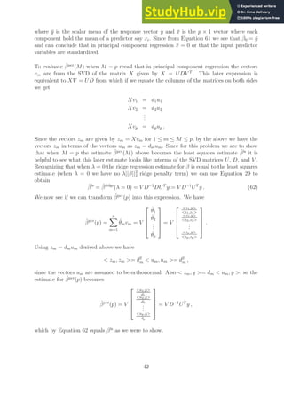
Ex. 3.13 (principal component regression)
Recall that principal component regression (PCR) using M components, estimates coeffi-
cients θ̂m, based on the top M largest variance principal component vectors zm. As such it
has a expression given by
ŷpcr
(M) = ȳ1 +
M
X
m=1
θ̂mzm (60)
= ȳ1 + X
M
X
m=1
θ̂mvm ,
using the fact that zm = Xvm and writing the fitted value under PCR as a function of the
number of retained components M. The above can be written in matrix form involving the
data matrix as
ŷpcr
(M) =
1 X
ȳ
PM
m=1 θ̂mvm
.
We can write this as the matrix
1 X
times a vector β̂pcr
if we take this later vector as
β̂pcr
(M) =
ȳ
PM
m=1 θ̂mvm
. (61)
This is the same as the books equation 3.62 when we restrict to just the last p elements of
β̂pcr
. It can be shown (for example in [10]) that for multiple linear regression models the
estimated regression coefficients in the vector β̂ can be split into two parts a scalar β̂0 and
a p × 1 vector β̂∗
as
β̂ =
β̂0
β̂∗
.
In addition the coefficient β̂0 can be shown to be related to β̂∗
as
β̂0 = ȳ − β̂∗
x̄ ,
41](https://image.slidesharecdn.com/asolutionmanualandnotesfortheelementsofstatisticallearning-230807171037-5c97f6ed/85/A-Solution-Manual-and-Notes-for-The-Elements-of-Statistical-Learning-pdf-41-320.jpg)

![otherwise. Now since all the vectors xj and x̃j are orthonormal we have
||y − ŷ||2
2 = ||y − Xβ̂||2
2 =
p
X
j=1
β̂j(1 − Ij)xj +
N
X
j=p+1
γjx̃j
2
2
=
p
X
j=1
β̂2
j (1 − Ij)2
||xj||2
2 +
N
X
j=p+1
γj
2
||x̃j||2
2
=
p
X
j=1
β̂2
j (1 − Ij)2
+
N
X
j=p+1
γj
2
.
Thus to minimize ||y − ŷ||2
2 we would pick the M values of Ij to be equal to one that have
the largest β̂2
j values. This is equivalent to sorting the values |β̂j| and picking the indices of
the largest M of these to have Ij = 1. All other indices j would be taken to have Ij = 0.
Using an indicator function this is equivalent to the expression
ˆ
βj
best−subset
= β̂jI[rank(|β̂j|) ≤ M] . (65)
For ridge regression, since X has orthonormal columns we have
β̂ridge
= (XT
X + λI)−1
XT
y
= (I + λI)−1
XT
y =
1
1 + λ
XT
y
=
1
1 + λ
β̂ls
,
which is the desired expression.
For the lasso regression procedure we pick the values of βj to minimize
RSS(β) = (y − Xβ)T
(y − Xβ) + λ
p
X
j=1
|βj| .
Expanding ŷ as ŷ =
Pp
j=1 βjxj and with y expressed again as in Equation 64 we have that
RSS(β) in this case becomes
RSS(β) =
p
X
j=1
(β̂j − βj)xj +
N
X
j=p+1
γjx̃j
2
2
+ λ
p
X
j=1
|βj|
=
p
X
j=1
(β̂j − βj)2
+
N
X
j=p+1
γ2
j + λ
p
X
j=1
|βj|
=
p
X
j=1
{(β̂j − βj)2
+ λ|βj|} +
N
X
j=p+1
γ2
j .
We can minimize this expression for each value of βj for 1 ≤ j ≤ p independently. Thus our
vector problem becomes that of solving p scalar minimization problems all of which look like
β∗
= argminβ
n
(β̂ − β)2
+ λ|β|
o
. (66)
45](https://image.slidesharecdn.com/asolutionmanualandnotesfortheelementsofstatisticallearning-230807171037-5c97f6ed/85/A-Solution-Manual-and-Notes-for-The-Elements-of-Statistical-Learning-pdf-45-320.jpg)

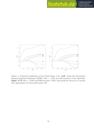
![as in performed in dup OSE all subset.R for the prostate data set. One could drop some
variables from the spam data to produce a smaller set of variables and then run such an
exhaustive search procedure if desired. The fact that we can run the other routines on this
problem is an argument for their value. When the above codes are run we obtain Table 4
comparing their performance.
LS Ridge Lasso PCR PLS
Test Error 0.121 0.117 0.123 0.123 0.119
Std Error 0.007 0.004 0.007 0.007 0.005
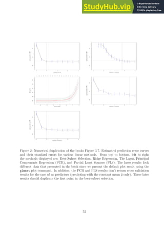
Table 4: Duplicated results for the books Table 3.3 but applied to the spam data set. Note
that ridge regression and partial least squares outperforms ordinary least squares.
Ex. 3.18 (conjugate gradient methods)
The conjugate gradient method is an algorithm that can be adapted to find the minimum
of nonlinear functions [8]. It also provides a way to solve certain linear algebraic equations
of the type Ax = b by formulating them as a minimization problem. Since the least squares
solution β̂ is given by the solution of a quadratic minimization problem given by
β̂ = argminβRSS(β) = argminβ(y − Xβ)T
(y − Xβ) . (67)
which has the explicit solution given by the normal equations or
(XT
X)β = XT
Y . (68)
One of the properties of the conjugate gradient algorithm is that when it is used to solve
Ax = b where x is an p × 1 vector it will terminate with the exact solution after p iterations.
Thus during is operation we get a sequence of p approximate values of the solution vector x.
One obvious way to use the conjugate gradient algorithm to derive refined estimates of β̂
the least squared solution is to use this algorithm to solve the normal Equations 68. Thus
after finishing each iteration of the conjugate gradient algorithm we have a new approximate
value of β̂(m)
for m = 1, 2, · · · , p and when m = p this estimate β̂(p)
corresponds to the least
squares solution. The value of m is a model selection parameter and can be selected by
cross validation. To derive the algorithm just described one would then need to specify the
conjugate gradient algorithm so that it was explicitly solving the normal Equations 68.
Warning: The problem with the statements just given is that while viewing the conjugate
gradient algorithm as a iterative algorithm to compute β̂ seems to be a reasonable algorithm,
the algorithm given in the book for partial least squares does not seem to be computing
iterative estimates for β̂LS
but instead each iteration seems to be computing an improved
estimates of y. While these two related as ŷ(m)
= Xβ̂(m)
, I don’t see how to modify the partial
least squares algorithm presented in the book into one that is approximating β̂. If anyone
sees a simple way to do this or knows of a paper/book that describes this transformation
please let the authors know.
47](https://image.slidesharecdn.com/asolutionmanualandnotesfortheelementsofstatisticallearning-230807171037-5c97f6ed/85/A-Solution-Manual-and-Notes-for-The-Elements-of-Statistical-Learning-pdf-47-320.jpg)
 .
The matrix in the middle of the above is a diagonal matrix with elements
d2
j
(d2
j +λ)2 . Thus
||β̂ridge
||2
2 =
p
X
i=1
d2
j (UT
y)j
2
(d2
j + λ)2
.
Where (UT
y)j is the jth component of the vector UT
y. As λ → 0 we see that the fraction
d2
j
(d2
j +λ)2 increases, and because ||β̂ridge
||2
2 is made up of sum of such terms, it too must increase
as λ → 0.
To determine if the same properties hold For the lasso, note that in both ridge-regression
and the lasso can be represented as the minimization problem
β̂ = argminβ
N
X
i=1
yi − β0 −
p
X
j=1
xijβj
!2
(69)
subject to
X
j
|βj|q
≤ t .
When q = 1 we have the lasso and when q = 2 we have ridge-regression. This form of the
problem is equivalent to the Lagrangian from given by
β̂ = argminβ
N
X
i=1
yi − β0 −
p
X
j=1
xijβj
!2
+ λ
p
X
j=1
|βj|q
. (70)
Because as λ → 0 the value of
P
|βj|q
needs to increase to have the product λ
P
|βj|q
stay constant and have the same error minimum value in Equation 70. Thus there is an
inverse relationship between λ and t in the two problem formulations, in that as λ decreases
t increases and vice versa. Thus the same behavior of t and
P
j |βj|q
with decreasing λ will
show itself in the lasso. This same conclusion can also be obtained by considering several of
the other properties of the lasso
• The explicit formula for the coefficients β̂j estimated by the lasso when the features
are orthogonal is given. In that case it equals sign(β̂j)(|β̂j|−λ)+. From this expression
we see that as we decrease λ we increase the value of β̂j, and correspondingly the norm
of the vector β̂.
48](https://image.slidesharecdn.com/asolutionmanualandnotesfortheelementsofstatisticallearning-230807171037-5c97f6ed/85/A-Solution-Manual-and-Notes-for-The-Elements-of-Statistical-Learning-pdf-48-320.jpg)


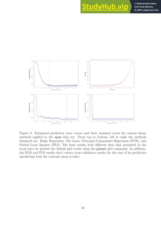
![made during the derivation of LDA in that the cut classification threshold point or the scalar
value of the expression
1
2
µ̂T
2 Σ̂−1
µ̂2 −
1
2
µ̂T
1 Σ̂−1
µ̂1 + log
N1
N
− log
N2
N
, (73)
is only Bayes optimal when the two class conditional densities are Gaussian and have the
same covariance matrix. Thus the conclusion suggested by the authors is that one might
be able to improve classification by specifying a different value for this cut point. In the R
function entitled two class LDA with optimal cut point.R we follow that suggestion and
determine the cut point that minimizes the classification error rate over the training set. We
do this by explicitly enumerating several possible cut points and evaluating the in-sample
error rate of each parametrized classifier1
. To determine the range of cut point to search for
this minimum over, we first estimate the common covariance matrix Σ̂, and the two class
means µ̂1 and µ̂2 in the normal ways and then tabulate (over all of the training samples x)
the left-hand-side of the book’s equation 4.11 or
xT
Σ̂−1
(µ̂2 − µ̂1) . (74)
Given the range of this expression we can sample cut points a number of times between
the minimum and maximum given value, classify the points with the given cut point and
estimating the resulting classifier error rate. The above code then returns the cut point
threshold that produces the minimum error rate over the in-sample data. This code is exer-
cised using the R script two class LDA with optimal cut point run.R where we perform
pairwise classification on two vowels. While the book claimed that this method is often su-
perior to direct use of LDA running the above script seems to indicate that the two methods
are very comparable. Running a pairwise comparison between the optimal cut point method
shows that it is only better then LDA 0.29 of the time. Additional tests on different data
sets is certainly needed.
Regularized Discriminant Analysis
Some R code for performing regularized discriminant analysis can be found in rda.R. This
code is exercised (on the vowel data) in the R code dup fig 4 7.R which duplicates the plot
given in the book. When that script is run we get
[1] Min test error rate= 0.478355; alpha= 0.969697
and the plot shown in Figure 10. This plot matches well with the one given in the book. In
addition, we can shrink Σ̂ towards a scalar and consider the more general three term model
Σ̂k(α, γ) = αΣ̂k + (1 − α)(γΣ̂ + (1 − γ)σ̂2
I) .
With this form for Σ̂k we can again run a grid search over the parameters α and γ and
select values that optimize out of sample performance. When we do that (at the bottom of
the dup fig 4 7.R) we get
1
A better algorithm but one that requires more computation would be to specify the classification point
and estimate the error rate using leave-one-out cross-validation.
60](https://image.slidesharecdn.com/asolutionmanualandnotesfortheelementsofstatisticallearning-230807171037-5c97f6ed/85/A-Solution-Manual-and-Notes-for-The-Elements-of-Statistical-Learning-pdf-60-320.jpg)
![0.0 0.2 0.4 0.6 0.8 1.0
0.0
0.1
0.2
0.3
0.4
0.5
0.6
Duplication of Figure 4.7
alpha
error
rate
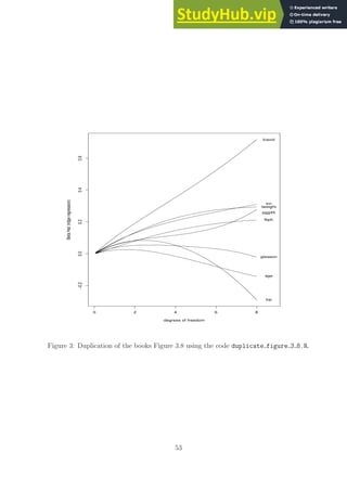
Figure 10: Duplication of the books Figure 4.7 using the code dup fig 4 7.R.
[1] Min test error rate= 0.439394; alpha= 0.767677; gamma= 0.050505
Notes on duplication of Table 4.1
In this dup table 4 1.R we call various R functions created to duplicate the results in the
book from Table 4.1. This code uses the R routine linear regression indicator matrix.R
which does classification based on linear regression (as presented in the introduction to this
chapter). When we run that code we get results given by
61](https://image.slidesharecdn.com/asolutionmanualandnotesfortheelementsofstatisticallearning-230807171037-5c97f6ed/85/A-Solution-Manual-and-Notes-for-The-Elements-of-Statistical-Learning-pdf-61-320.jpg)
![Technique Training Test
[1] Linear Regression: 0.477273; 0.666667
[1] Linear Discriminant Analysis (LDA): 0.316288; 0.556277
[1] Quadratic Discriminant Analysis (QDA): 0.011364; 0.528139
[1] Logistic Regression: 0.221591; 0.512987
These results agree well with the ones given in the book.
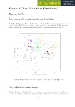
Notes on Reduced-Rank Linear Discriminant Analysis
1 2 3 4
0
1
2
3
4
5
6
Coordinate 1 for Training Data
Coordinate
2
for
Training
Data
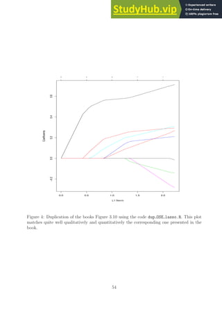
Figure 11: Duplication of the coordinate 1 - 7 projection found in the books Figure 4.8.
In this section of these notes we implement the reduced-rank linear discriminant analysis in
the R code reduced rank LDA.R. Using this code in the R code dup fig 4 8.R we can then
duplicate the projections presented in figure 4.8 from the book. When we run that code we
get the plot given in Figure 11. This plot matches the results in the book quite well. In the
R code dup fig 4.10.R we have code that duplicates figure 4.10 from the book. When that
code is run we get the plot shown in Figure 12.
62](https://image.slidesharecdn.com/asolutionmanualandnotesfortheelementsofstatisticallearning-230807171037-5c97f6ed/85/A-Solution-Manual-and-Notes-for-The-Elements-of-Statistical-Learning-pdf-62-320.jpg)
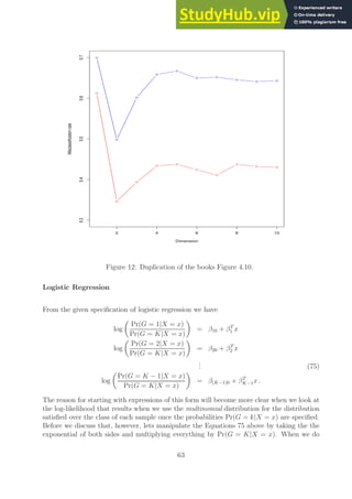


![Notes on Optimal Separating Hyperplanes
For the Lagrange (primal) function to be minimized with respect to β and β0 given by
LP =
1
2
||β||2
−
N
X
i=1
αi[yi(xT
i β + β0) − 1] , (82)
we have derivatives (set equal to zero) given by
∂Lp
∂β
= β −
N
X
i=1
αiyixi = 0 (83)
∂Lp
∂β0
= 0 −
N
X
i=1
αiyi = 0 . (84)
Note that by expanding we can write Lp as
Lp =
1
2
||β||2
−
N
X
i=1
αiyixT
i β − β0
N
X
i=1
αiyi +
N
X
i=1
αi .
From Equation 84 the third term in the above expression for Lp is zero. Using Equation 83
to solve for β we find that the first term in the above expression for Lp is
||β||2
= βT
β =
N
X
i=1
αiyixT
i
! N
X
j=1
αjyjxj
!
=
N
X
i=1
N
X
j=1
αiαjyiyjxT
i xj ,
and that the second terms in the expression for Lp is
N
X
i=1
αiyixT
i β =
N
X
i=1
αiyixT
i
N
X
j=1
αjyjxj
!
=
N
X
i=1
N
X
j=1
αiαjyiyjxT
i xj .
Thus with these two substitutions the expression for Lp becomes (we now call this LD)
LD =
N
X
i=1
αi −
1
2
N
X
i=1
N
X
j=1
αiαjyiyjxT
i xj . (85)
Exercise Solutions
Ex. 4.1 (a constrained maximization problem)
To solve constrained maximization or minimization problems we want to use the idea of
Lagrangian multipliers. Define the Lagrangian L as
L(a; λ) = aT
Ba + λ(aT
Wa − 1) .
67](https://image.slidesharecdn.com/asolutionmanualandnotesfortheelementsofstatisticallearning-230807171037-5c97f6ed/85/A-Solution-Manual-and-Notes-for-The-Elements-of-Statistical-Learning-pdf-67-320.jpg)


![Chapter 5 (Basis Expansions and Regularization)
Notes on the Text
There is a nice chapter on using B-splines in the R language for regression problems in the
book [11]. There are several regression examples using real data and a discussion of the
various decisions that need to be made when using splines for regression. The chapter also
provides explicit R code (and discussions) demonstrating how to solve a variety of applied
regression problems using splines.
Notes on piecewise polynomials and splines
If the basis functions hm(X) are local piecewise constants i.e. if
h1(X) = I(X ξ1) , h2(X) = I(ξ1 ≤ X ξ2) , h3(X) = I(ξ2 ≤ X) ,
and taking our approximation to f(X) of
f(X) ≈
3
X
m=1
βmhm(X) ,
then the coefficients βm are given by solving the minimization problem
β = ArgMinβ f(X) −
3
X
m=1
βmhm(X)
2
= ArgMinβ
Z
f(x) −
3
X
m=1
βmhm(X)
!2
dX
= ArgMinβ
Z ξ1
ξL
(f(X) − β1)2
dX +
Z ξ2
ξ1
(f(X) − β2)2
dX +
Z ξR
ξ2
(f(X) − β3)2
dX
.
Here ξL and ξR are the left and right end points of the functions domain. Since the above is
a sum of three positive independent (with respect to βm) terms we can minimize the total
sum by minimizing each one independently. For example, we pick β1 that minimizes the first
term by taking the derivative of that term with respect to β1, and setting the result equal
to zero and solving for β1. We would have
d
dβ1
Z ξ1
ξL
(f(X) − β1)2
dX = 2
Z ξ1
ξL
(f(X) − β1)dX = 0 .
When we solving this for β1 we get
β1 =
1
ξ1 − ξL
Z ξ1
ξL
f(X)dX = Y 1 ,
as claimed by the book. The other minimizations over β2 and β3 are done in the same way.
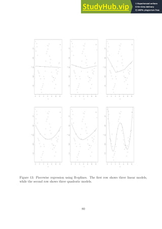
78](https://image.slidesharecdn.com/asolutionmanualandnotesfortheelementsofstatisticallearning-230807171037-5c97f6ed/85/A-Solution-Manual-and-Notes-for-The-Elements-of-Statistical-Learning-pdf-78-320.jpg)


![[1] err_rate_train= 0.093114; err_rate_test= 0.24374
These numbers are not that different for the ones given in the book. If we train a quadratic
discriminant classifier on these two phonemes we get
[1] err_rate_train= 0.000000; err_rate_test= 0.33941
Finally, just to compare algorithms performance, we can fit (using cross validation) a regu-
larized discriminant analysis model where we find
[1] err_rate_train= 0.075781; err_rate_test= 0.19590
the optimal parameters found were α = 0.1111111 and γ = 0.7474747. While this testing
error rate is not as good as the regularized result the book gives 0.158 regularized discriminant
analysis gives the best result of the three classifiers tested.
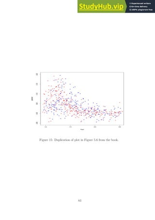
Notes on the bone mineral density (smoothing splines example)
In the R code dup fig 5 6.R we duplicate some of the plots shown in the book. When we
run that script we get the two plots shown in Figure 15. This plot uses the R command
smooth.spline.
Exercise Solutions
Ex. 5.9 (deriving the Reinsch form)
Given
Sλ = N(NT
N + λΩN )−1
NT
,
when N is invertible then we have
Sλ = (N−T
(NT
N + λΩN )N−1
)−1
= (N−T
NT
NN−1
+ λN−T
ΩN N−1
)−1
= (I + λN−T
ΩN N−1
)−1
,
so K ≡ N−T
ΩN N−1
.
82](https://image.slidesharecdn.com/asolutionmanualandnotesfortheelementsofstatisticallearning-230807171037-5c97f6ed/85/A-Solution-Manual-and-Notes-for-The-Elements-of-Statistical-Learning-pdf-82-320.jpg)
![Chapter 7 (Model Assesment and Selection)
Notes on the Text
Note: This chapter needs to be proofed.
Notes on the bias-variance decomposition The true model is Y = f(X) + ǫ with E(ǫ) = 0
and Var(ǫ) = σ2
ǫ . Define Err(x0) as the test error we are after is generaliztaion error i.e. how
well we will do on samples from outside the given data set.
Err(x0) = E[(Y − ˆ
f(x0))2
|X = x0]
= E[(f(x0) + ǫ − ˆ
f(x0))2
|X = x0]
= E[(f(x0) − ˆ
f(x0))2
+ 2ǫ(f(x0) − ˆ
f(x0)) + ǫ2
|X = x0]
= E[(f(x0) − ˆ
f(x0))2
|X = x0]
+ 2E[ǫ(f(x0) − ˆ
f(x0))|X = x0]
+ E[ǫ2
|X = x0] .
Now
E[ǫ(f(x0) − ˆ
f(x0))|X = x0] = E[ǫ|X = x0]E[(f(x0) − ˆ
f(x0))|X = x0] = 0 .
and so the above becomes
Err(x0) = σ2
ǫ + E[(f(x0) − ˆ
f(x0))2
|X = x0] .
Now ˆ
f is also random since it depends on the random selection of the initial training set.
To evalaute this term we can consider the expected value of ˆ
f(x0) taken over all random
training sets. We have
E[(f(x0) − ˆ
f(x0))2
|X = x0] = E[(f(x0) − E ˆ
f(x0) + E ˆ
f(x0) − ˆ
f(x0))2
|X = x0] .
This later expression expands to
E[(f(x0) − E ˆ
f(x0))2
+ 2(f(x0) − E ˆ
f(x0))(E ˆ
f(x0) − ˆ
f(x0)) + (E ˆ
f(x0) − ˆ
f(x0))2
] .
Note f(x0) and E ˆ
f(x0) given X = x0 are not random since f(x0) in our universie output
and E ˆ
f(x0) has already taken the expectation. Thus when we take the expectation of the
above we get
E[E ˆ
f(x0) − ˆ
f(x0)|X = x0] = 0 ,
and the second term in the above vanishes. We end with
E[(f(x0) − ˆ
f(x0))2
|X = x0] = (f(x0) − E ˆ
f(x0))2
+ E[(E ˆ
f(x0) − ˆ
f(x0))2
]
= σ2
ǫ + model bias2
+ model variance .
84](https://image.slidesharecdn.com/asolutionmanualandnotesfortheelementsofstatisticallearning-230807171037-5c97f6ed/85/A-Solution-Manual-and-Notes-for-The-Elements-of-Statistical-Learning-pdf-84-320.jpg)
![Y = f(X) + ǫ Var(ǫ) = σ2
ǫ
Err(x0) = E[(Y − ˆ
f(x0))2
|X = x0]
= E[(f(x) + ǫ − ˆ
f(x0))2
|X = x0]
= E[(f(x) − ˆ
f(x0) + ǫ)2
|X = x0]
= E[(f(x0) − Ef(x0) + Ef(x0) − ˆ
f(x0) + ǫ)2
]
= E[(f(x0) − Ef(x0))2
+ 2(f(x0) − Ef(x0))(Ef(x0) − ˆ
f(x0)) + (Ef(x0) − ˆ
f(x0))2
+ ǫ2
]
We take the expectation over possible Y values via ǫ variabliligy and possible training sets
that go into constants of ˆ
f(x0). Note that all E[(·)ǫ] = E[(·)]E[ǫ] = 0. The middle terms
vanishes since E[f(x0) − Ef(x0)] = 0.
Introduce E[ ˆ
f(x0)] expected value over all training sets predicition using the median
For k nearest neighbor
ˆ
f(x0) =
1
k
k
X
l=1
f(x(l))
≈
1
k
k
X
l=1
(f(x0) + ε(l)) = f(x0) +
1
k
k
X
l=1
ε(l) .
Now the variance of the estimate ˆ
f(x0) comes from the 1
k
Pk
l=1 ε(k) random term. Taking
the variance of this summation we have
1
k2
k
X
l=1
Var(ε(l)) =
1
k2
kVar(ε)
1
k
σ2
ε . (102)
Which is the equation in the book.
ˆ
fp(x) = β̂T
x we have
Err(x0) = E[(Y − ˆ
fp(x0))2
|X = x0]
= σ2
ε + [f(x0) − E ˆ
fp(x0)]2
+ ||h(x0||2
σ2
ε .
ˆ
fp(x0) = xT
0 (XT
X)−1
XT
y where y is random since y = y0 + ε
1
N
X
Err(x0) = σ2
ε +
1
N
N
X
i=1
[f(xi) − E ˆ
f(xi)]2
+
p
N
σ2
ε . (103)
85](https://image.slidesharecdn.com/asolutionmanualandnotesfortheelementsofstatisticallearning-230807171037-5c97f6ed/85/A-Solution-Manual-and-Notes-for-The-Elements-of-Statistical-Learning-pdf-85-320.jpg)
![Chapter 10 (Boosting and Additive Trees)
Notes on the Text
Notes on the Sample Classification Data
For AdaBoost.M1 the books suggests using a “toy” ten-dimensional data set where the
individual elements X1, X2, · · · , X10 of the vector X are standard independent Gaussian
random draws and the classification labels (taken from {−1, +1}) are assigned as
Y =
+1 if
P10
j=1 X2
j χ2
10(0.5)
−1 otherwise
.
Here χ2
10(0.5) is the median of a chi-squared random variable with 10 degrees of freedom.
In [2] it is stated that the Xi are standard independent Gaussian and their 10 values are
squared and then summed one gets a chi-squared random variable (by definition) with 10
degrees of freedom. Thus the threshold chosen of χ2
10(0.5) since it is the median will split
the data generated exactly (in the limit of infinite samples) into two equal sets. Thus when
we ask for N samples we approximately equal number of N
2
of samples in each class and
it is a good way to generate testing data. Code to generate data from this toy problem
in Matlab is given by the function gen data pt b.m and in the R language in the function
gen eq 10 2 data.R.
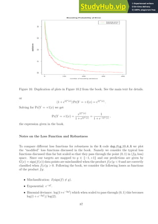
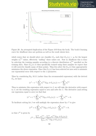
Notes on duplicated Figure 10.2
See the R code dup fig 10 2.R where we use the R package gbm do duplicate the books
Figure 10.2. That package has an option (distribution=’adaboost’) that will perform
gradient boosting to minimize the exponential adaboost loss function. Since this package
does gradient boosting (a more general form of boosting) to get the results from the book
one needs to set the learning rate to be 1. When that code is run we get the results given in
Figure 16, which matches quite well the similar plot given in the text. For a “home grown”
Matlab implementation of AdaBoost see the problem on Page 94.
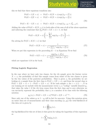
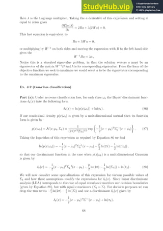
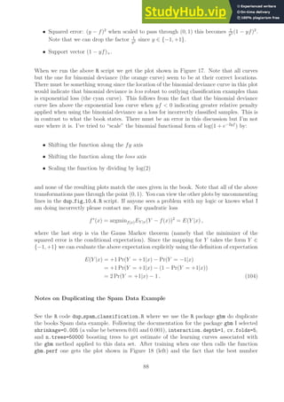
Notes on Why Exponential Loss
From the text and Equation 105 we have
f∗
(x) = argminf(x)EY |x(e−Y f(x)
) =
1
2
log
Pr(Y = +1|x)
Pr(Y = −1|x)
Solving the above for Pr(Y = +1|x) in terms of f∗
(x) we first write the above as
Pr(Y = +1|x)
1 − Pr(Y = +1|x)
= e2f∗(x)
,
86](https://image.slidesharecdn.com/asolutionmanualandnotesfortheelementsofstatisticallearning-230807171037-5c97f6ed/85/A-Solution-Manual-and-Notes-for-The-Elements-of-Statistical-Learning-pdf-86-320.jpg)
![−2 −1 0 1 2
0.0
0.5
1.0
1.5
2.0
2.5
3.0
y f
loss
Figure 17: An attempted duplication of plots in Figure 10.4 from the book. See the main
text for details.
of boosting trees is 10563. The error rate with this tree is 5.14%. This is a bit larger
than the numbers reported in the book but still in the same ballpark. If we retrain with
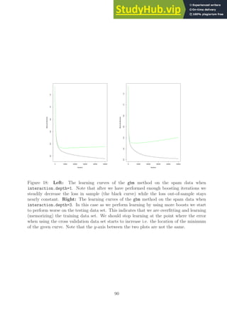
interaction.depth=3 we get the learning curve given in Figure 18 (right). The optimal
number of boosting trees in this case 7417, also given a smaller testing error of 4.75%. The
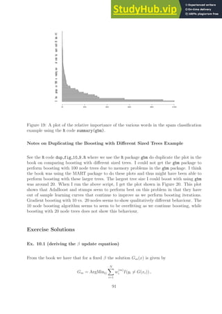
R routine summary can be use to plot a relative importance graph. When we do that we get
the plot shown in Figure 19.
While the labeling of the above plot is not as good in the books we can print the first twenty
most important words (in the order from most important to less important) to find
most_important_words[1:20]
[1] $ !
[3] remove free
[5] hp your
[7] capital_run_length_average capital_run_length_longest
[9] george capital_run_length_total
[11] edu money
[13] our you
[15] internet 1999
[17] will email
[19] re receive
This ordering of words that are most important for the classification task agrees very well
with the ones presented in the book.
89](https://image.slidesharecdn.com/asolutionmanualandnotesfortheelementsofstatisticallearning-230807171037-5c97f6ed/85/A-Solution-Manual-and-Notes-for-The-Elements-of-Statistical-Learning-pdf-89-320.jpg)

![0 50 100 150 200 250 300 350 400
0.1
0.15
0.2
0.25
0.3
0.35
0.4
0.45
0.5
training err
testing err
Figure 21: A duplication of the Figure 10.2 from the book.
Ex. 10.4 (Implementing AdaBoost with trees)
Part (a): Please see the web site for a suite of codes that implement AdaBoost with trees.
These codes were written by Kelly Wallenstein under my guidance.
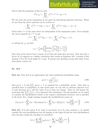
Part (b): Please see the Figure 21 for a plot of the training and test error using the provide
AdaBoost Matlab code and the suggested data set. We see that the resulting plot looks very
much like the on presented in Figure 10.2 of the book helping to verify that the algorithm
is implemented correctly.
Part (c): I found that the algorithm proceeded to run for as long as I was able to wait.
For example, Figure 21 has 800 boosting iterations which took about an hour train and test
with the Matlab code. As the number of boosting iterations increased I did not notice any
significant rise in the test error. This was one of the purported advantages of the AdaBoost
algorithm.
Ex. 10.5 (Zhu’s multiclass exponential loss function)
Part (a): We want to find the vector function f∗
(x) such that
f∗
(x) = argminf(x)EY |x[L(Y, f)] = argminf(x)EY |x
exp
−
1
K
Y T
f
,
94](https://image.slidesharecdn.com/asolutionmanualandnotesfortheelementsofstatisticallearning-230807171037-5c97f6ed/85/A-Solution-Manual-and-Notes-for-The-Elements-of-Statistical-Learning-pdf-94-320.jpg)
![and where the components of f(x) satisfy the constraint
PK
k=1 fk(x) = 0. To do this we will
introduce the Lagrangian L defined as
L(f; λ) ≡ EY |x
exp
−
1
K
Y T
f
− λ
K
X
k=1
fk − 0
!
.
Before applying the theory of continuous optimization to find the optima of L we will first
evaluate the expectation
E ≡ EY |x
exp
−
1
K
Y T
f
.
Note that by expanding the inner products the above expectation can be written as
EY |x
exp
−
1
K
(Y1f1 + Y2f2 + · · · + YK−1fK−1 + YKfK
.
We then seek to evaluate the above expression by using the law of the unconscious statistician
E[f(X)] ≡
X
f(xi)p(xi) .
In the case we will evaluate the above under the encoding for the vector Y given by
Yk =
1 k = c
− 1
K−1
k 6= c
.
This states that when the true class of our sample x is from the class c, the response vector
Y under this encoding has a value of 1 in the c-th component and the value − 1
K−1
in all
other components. Using this we get the conditional expectation given by
E = exp
−
1
K
−
1
K − 1
f1(x) + f2(x) + · · · + fK−1(x) + fK(x)
Prob(c = 1|x)
+ exp
−
1
K
f1(x) −
1
K − 1
f2(x) + · · · + fK−1(x) + fK(x)
Prob(c = 2|x)
.
.
.
+ exp
−
1
K
f1(x) + f2(x) + · · · −
1
K − 1
fK−1(x) + fK(x)
Prob(c = K − 1|x)
+ exp
−
1
K
f1(x) + f2(x) + · · · + fK−1(x) −
1
K − 1
fK(x)
Prob(c = K|x) .
Now in the exponential arguments in each of the terms above by using the relationship
−
1
K − 1
=
K − 1 − K
K − 1
= 1 −
1
K − 1
,
we can write the above as
E = exp
−
1
K
f1(x) + f2(x) + · · · + fK−1(x) + fK(x) −
K
K − 1
f1(x)
Prob(c = 1|x)
+ exp
−
1
K
f1(x) + f2(x) + · · · + fK−1(x) + fK(x) −
K
K − 1
f2(x)
Prob(c = 2|x)
.
.
.
+ exp
−
1
K
f1(x) + f2(x) + · · · + fK−1(x) + fK(x) −
K
K − 1
fK−1(x)
Prob(c = K − 1|x)
+ exp
−
1
K
f1(x) + f2(x) + · · · + fK−1(x) + fK(x) −
K
K − 1
fK(x)
Prob(c = K|x) .
95](https://image.slidesharecdn.com/asolutionmanualandnotesfortheelementsofstatisticallearning-230807171037-5c97f6ed/85/A-Solution-Manual-and-Notes-for-The-Elements-of-Statistical-Learning-pdf-95-320.jpg)


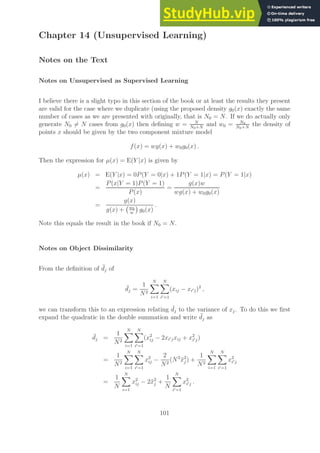


![Setting this equal to zero and solving for µ we find
µ = x̄ − Vq
1
N
N
X
i=1
λi
!
, (116)
where x̄ = 1
N
PN
i=1 xi. Next we take the derivative of Equation 115, with respect to λi, set
the result equal to zero and then solve for λi. To do this we write the sum in Equation 115
as
N
X
i=1
[(xi − µ)T
− 2(xi − µ)T
Vqλi + λT
i V T
q Vqλi] .
From which we see that taking, the ∂
∂λi
derivative of this expression and setting the result
equal to zero is given by
−2((xi − µ)T
Vq)T
+ +(V T
q Vq + V T
q Vq)λi = 0 ,
or
V T
q (xi − µ) = V T
q Vqλi = λi , (117)
since V T
q Vq = Ip. When we put this value of λi into Equation 116 to get
µ = x̄ − VqV T
q (x̄ − µ) .
Thus µ must satisfy
VqV T
q (x̄ − µ) = x̄ − µ ,
or
(I − VqV T
q )(x̄ − µ) = 0 .
Now I − VqV T
q is the orthogonal projection onto the subspace spanned by the columns of Vq
thus µ = x̄ + h, where h is an arbitray p dimensional vector in the subspace spanned by Vq.
Since Vq has a rank of q the vector h is selected from an p − q dimensional space (the space
spanned by the orthogonal complement of the columns of Vq). If we take h = 0 then µ = x̄
and we get
λi = V T
q (xi − x̄) ,
from Equation 117.
Ex. 14.8 (the procrustes transformation)
For the Procrustes transformation we want to evaluate
argminµ,R||X2 − (X1R + 1µT
)||F . (118)
This has the same solution when we square the same norm as above
argminµ,R||X2 − (X1R + 1µT
)||2
F .
When we use the fact that ||X||2
F = trace(XT
X) we see that the above norm equals
trace((X2 − X1R − 1µT
)T
(X2 − X1R − 1µT
)) .
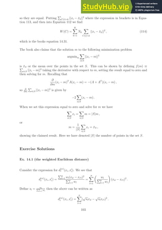
105](https://image.slidesharecdn.com/asolutionmanualandnotesfortheelementsofstatisticallearning-230807171037-5c97f6ed/85/A-Solution-Manual-and-Notes-for-The-Elements-of-Statistical-Learning-pdf-105-320.jpg)
![when we solve for R we get
R = (X̃T
1 X̃1)−1
(X̃T
1 X̃2) . (121)
Warning: this result is different that what is claimed in the book and I don’t see how to
make the two the same. If anyone knows how to make the results equivalent please let me
know. One piece of the puzzel is that R is supposted to be orthogonal. I have not explicitly
enforeced this constraint in any way. I think I need to modify the above minimization to
add the constraint that RT
R = I.
This problem is discussed in greater detail in [9].
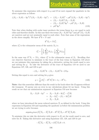
107](https://image.slidesharecdn.com/asolutionmanualandnotesfortheelementsofstatisticallearning-230807171037-5c97f6ed/85/A-Solution-Manual-and-Notes-for-The-Elements-of-Statistical-Learning-pdf-107-320.jpg)

![test error rate
l
e
arni
n
g
method
GBM−1
GBM−6
RF−1
RF−3
0.06 0.08 0.10 0.12 0.14 0.16
Figure 23: A duplication of the books Figure 15.2, comparing random forests with gradient
boosting on the “nested spheres” data.
Exercise Solutions
Ex. 15.1 (the variance of the mean of correlated samples)
We are told to assume that xi ∼ N(m, σ2
) for all i and that xi and xj are correlated with a
correlation coefficient of ρ. We first compute some expectation of powers of xi. First recall
from probability that the variance in terms of the moments is given by
E[X2
] = Var(X) + E[X]2
.
Next the definition of the correlation coefficient ρ we have that
1
σ2
E[(xi − m)(xj − m)] = ρ 0 .
We can expand the above expectation to get
E[xixj] = ρσ2
+ m2
.
Thus we now have shown that
E[xi] = m
E[xixj] =
ρσ2
+ m2
i 6= j
σ2
+ m2
i = j
.
The variance of the estimate of the mean is now given by
Var
1
B
X
xi
=
1
B2
Var
X
xi
=
1
B2
E
X
xi
2
− E
hX
xi
i2
109](https://image.slidesharecdn.com/asolutionmanualandnotesfortheelementsofstatisticallearning-230807171037-5c97f6ed/85/A-Solution-Manual-and-Notes-for-The-Elements-of-Statistical-Learning-pdf-109-320.jpg)
![The second expectation is easy to evaluate
E
hX
xi
i
=
X
E[xi] = Bm .
For the first expectation note that
n
X
i=1
xi
!2
=
X
i,j
xixj .
Thus we have
E
X
xi
2
=
X
i,j
E[xixj] = BE[x2
i ] + (B2
− B)E[xixj]
= B(σ2
+ m2
) + B(B − 1)(ρσ2
+ m2
)
= Bσ2
+ B2
ρσ2
− Bρm2
+ B2
m2
.
With this expression we can now compute Var 1
B
P
xi
and find
Var
1
B
X
xi
=
σ2
B
+ ρσ2
−
ρσ2
B
= ρσ2
+
1 − ρ
B
σ2
. (122)
Which matches the expression in the book.
110](https://image.slidesharecdn.com/asolutionmanualandnotesfortheelementsofstatisticallearning-230807171037-5c97f6ed/85/A-Solution-Manual-and-Notes-for-The-Elements-of-Statistical-Learning-pdf-110-320.jpg)
![A Appendix
A.1 Matrix and Vector Derivatives
In this section of the appendix we enumerate several matrix and vector derivatives that are
used in the previous document. We begin with some derivatives of scalar forms
∂xT
a
∂x
=
aT
x
∂x
= a (123)
∂xT
Bx
∂x
= (B + BT
)x . (124)
Next we present some derivatives involving traces. We have
∂
∂X
trace(AX) = AT
(125)
∂
∂X
trace(XA) = AT
(126)
∂
∂X
trace(AXT
) = A (127)
∂
∂X
trace(XT
A) = A (128)
∂
∂X
trace(XT
AX) = (A + AT
)X . (129)
Derivations of expressions of this form are derived in [3, 4].
111](https://image.slidesharecdn.com/asolutionmanualandnotesfortheelementsofstatisticallearning-230807171037-5c97f6ed/85/A-Solution-Manual-and-Notes-for-The-Elements-of-Statistical-Learning-pdf-111-320.jpg)
![References
[1] B. Abraham and J. Ledolter. Statistical Methods for Forecasting. Wiley, Toronto, 1983.
[2] M. H. DeGroot. Optimal Statistical Decisions. 2004.
[3] P. A. Devijver and J. Kittler. Pattern recognition: A statistical approach. Prentice Hall,
1982.
[4] P. S. Dwyer and M. S. Macphail. Symbolic matrix derivatives. Annals of Mathematical
Statistics, 19(4):517–534, 1948.
[5] J. H. Friedman, T. Hastie, and R. Tibshirani. Regularization paths for generalized linear
models via coordinate descent. Journal of Statistical Software, 33(1):1–22, 12 2009.
[6] T. Hastie, R. Tibshirani, and J. Friedman. The Elements of Statistical Learning.
Springer, New York, 2001.
[7] B.-H. Mevik and R. Wehrens. The pls package: Principal component and partial least
squares regression in R. Journal of Statistical Software, 18(2):1–24, 1 2007.
[8] J. Nocedal and S. J. Wright. Numerical Optimization. Springer, August 2000.
[9] P. Schnemann. A generalized solution of the orthogonal procrustes problem. Psychome-
trika, 31(1):1–10, 1966.
[10] S. Weisberg. Applied Linear Regression. Wiley, New York, 1985.
[11] D. Wright and K. London. Modern regression techniques using R: a practical guide for
students and researchers. SAGE, 2009.
112](https://image.slidesharecdn.com/asolutionmanualandnotesfortheelementsofstatisticallearning-230807171037-5c97f6ed/85/A-Solution-Manual-and-Notes-for-The-Elements-of-Statistical-Learning-pdf-112-320.jpg)

The document provides notes and solutions for exercises from the book "The Elements of Statistical Learning". It summarizes the key concepts in statistical decision theory and linear regression models. It then works through the derivations of important equations from the book, including the bias-variance decomposition of mean squared error. The document aims to help readers understand difficult concepts from the book and improve their learning through working on exercises.