Distributed Stochastic Gradient
MCMC
SungjinAhn1
Babak Shahbaba2
Max Welling3
1
Department of Computer Science, University of California, Irvine
2
Department of Statistics, University of California, Irvine
3
Machine Learning Group, University of Amsterdam
June 20, 2016
1 / 28
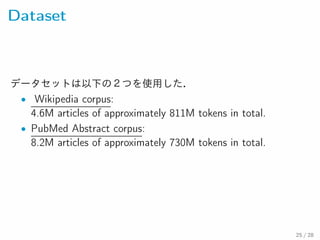
Distributed Inference inLDA
Approximate Distributed LDA (AD-LDA) [Newman et al, 2007]
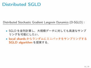
• MCMC にかかる計算時間を減らすため,それぞれの local
shard に周辺化ギブスサンプリングを行う手法.
• N
1回のサンプリングごとの計算コストが ( S ) まで減少.
• global states との同期により local copy の重みを修正できる.
13 / 28
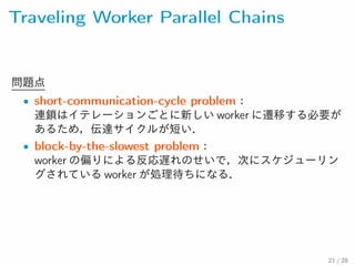
SGLD on PartitionedDatasets
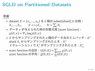
準備
• sudataset X = {x1,..., xN } を S 個の bset(shard) に分割:
X1,..., XS, X = ∪sXs, N =
∑
s Ns
• データ x が与えられた時の対数尤度 (score function):
g(θ; x) = ∇θ log p(θ; x)
• X からサンプリングされた n 個のデータ点のミニバッチ:X n
shard Xs からサンプリングされたとき:Xs
n
イ テレーション t で X n
s
がサンプリングされたとき:X n
s,t
• score function の合計:G(θ ; X ) =
∑
x∈X g(θ; x)
score function の平均:g¯(θ ; X ) = |X
1
|
G(θ; X)
17 / 28
18.
SGLD on PartitionedDatasets
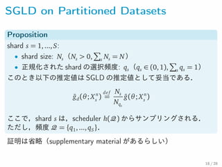
Proposition
shard s = 1,...,S:
• shard size: Ns(Ns > 0,
∑
s Ns = N)
• 正規化された shard の選択頻度: qs(qs ∈ (0, 1),
∑
s qs = 1)
このとき以下の推定値は SGLD の推定値として妥当である.
¯gd(θ; X n
s
)
de f
=
Ns
Nqs
¯g(θ; X n
s
)
ここで,shard s は,scheduler h( ) からサンプリングされる.ただ
し,頻度 = {q1,...,qS}.
証明は省略(supplementary material があるらしい)
18 / 28
19.
SGLD on PartitionedDatasets
流れ
(1) shard をサンプリングで選ぶ.
s ∼ h( ) = Category(q1,...,qS)
(2) 選んだ shard からミニバッチ X n
s
をサンプリングする.
(3) ミニバッチを使って score 平均 g¯(θ ; Xs
n ) 計算 .
(4) score 平均に N
N
q
s
s
をかけて,重みを修正する.
19 / 28
20.
SGLD on PartitionedDatasets
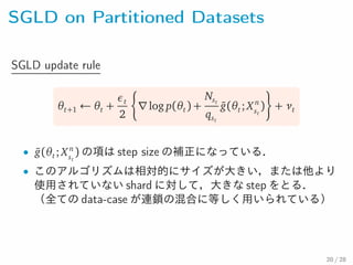
SGLD update rule
θt+1 ← θt +
εt
2
∇log p(θt) +
Nst
qst
¯g(θt; X n
st
) + νt
• ¯g(θt; X n
st
) の項は step size の補正になっている.
• このアルゴリズムは相対的にサイズが大きい,または他より使用
されていない shard に対して,大きな step をとる.(全ての
data-case が連鎖の混合に等しく用いられている)
20 / 28
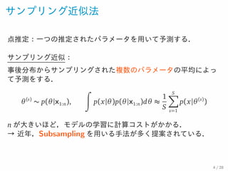
![Mini-batch-based MCMC
Stochastic Gradient Langevin Dynamics (SGLD)
[Welling & Teh, 2011]
• 単純な Stochastic gradient ascent を拡張する.
• MAP ではなく完全な事後分布からサンプリングするようなベ
イズ推定のアルゴリズムを考える.
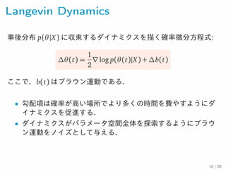
• Langevin Dynamics [Neal, 2010] は MCMC の手法の一つ.解
が単なる MAP に陥らないよう,パラメータの更新時にGaussian
noise を加える.
6 / 28](https://image.slidesharecdn.com/d-sgld-161107031537/85/Distributed-Stochastic-Gradient-MCMC-6-320.jpg)
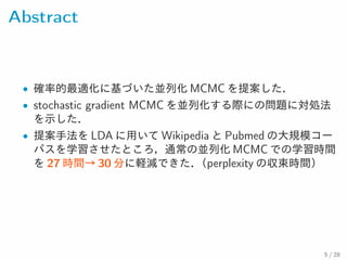
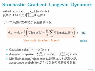
![Stochastic Gradient Ascent
確率的最適化アルゴリズム [Robbins & Monro, 1951]
At iterattion t = 1,2,... :
• データセットから subset {xt1,..., xtn} (n << N) をとる.
• subset を用いて対数事後分布の勾配の近似値を計算する.
∇log p(θt|X) ≈ ∇log p(θt) +
n
N
n∑
i=1
∇log p(xti|θt)
• この値を用いてパラメータの値を更新する.
θt+1 = θt +
εt
2
∇log p(θt) +
n
N
n∑
i=1
∇log p(xti|θt)
8 / 28](https://image.slidesharecdn.com/d-sgld-161107031537/85/Distributed-Stochastic-Gradient-MCMC-8-320.jpg)
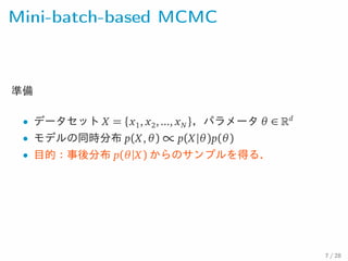
![Distributed Inference in LDA
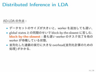
Approximate Distributed LDA (AD-LDA) [Newman et al, 2007]
• MCMC にかかる計算時間を減らすため,それぞれの local
shard に周辺化ギブスサンプリングを行う手法.
• N
1回のサンプリングごとの計算コストが ( S ) まで減少.
• global states との同期により local copy の重みを修正できる.
13 / 28](https://image.slidesharecdn.com/d-sgld-161107031537/85/Distributed-Stochastic-Gradient-MCMC-13-320.jpg)
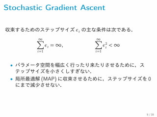
![Distributed Inference in LDA
Yahoo-LDA (Y-LDA) [Ahmed et al, 2012]
• 非同期での更新により,block-by-the-slowest の解決をした.
• 非同期で無限に更新するとパフォーマンスが悪化する.
[Ho et al, 2013]
15 / 28](https://image.slidesharecdn.com/d-sgld-161107031537/85/Distributed-Stochastic-Gradient-MCMC-15-320.jpg)

![比較手法
• AD-LDA
• Async-LDA (Y-LDA)
[Ahmed et al., 2012; Smola & Narayanamurthy, 2010]
• SGRLD: Stochastic gradient Riemannian Langevin dynamics
[Patterson & Teh, 2013)]
26 / 28](https://image.slidesharecdn.com/d-sgld-161107031537/85/Distributed-Stochastic-Gradient-MCMC-26-320.jpg)


![[DL輪読会]Scalable Training of Inference Networks for Gaussian-Process Models](https://cdn.slidesharecdn.com/ss_thumbnails/mainslideshare1-190927025239-thumbnail.jpg?width=640&height=640&fit=bounds)
![[DL輪読会]A Bayesian Perspective on Generalization and Stochastic Gradient Descent](https://cdn.slidesharecdn.com/ss_thumbnails/20171106dl2-171108033614-thumbnail.jpg?width=640&height=640&fit=bounds)


![[DL Hacks] Deterministic Variational Inference for RobustBayesian Neural Netw...](https://cdn.slidesharecdn.com/ss_thumbnails/adobepdffile2-190628001736-thumbnail.jpg?width=640&height=640&fit=bounds)


