Lecture2 xing

1. © Eric Xing @ CMU, 2006-2010 1
Machine Learning
Generative verses discriminative
classifier
Eric Xing
Lecture 2, August 12, 2010
Reading:

2. © Eric Xing @ CMU, 2006-2010 2
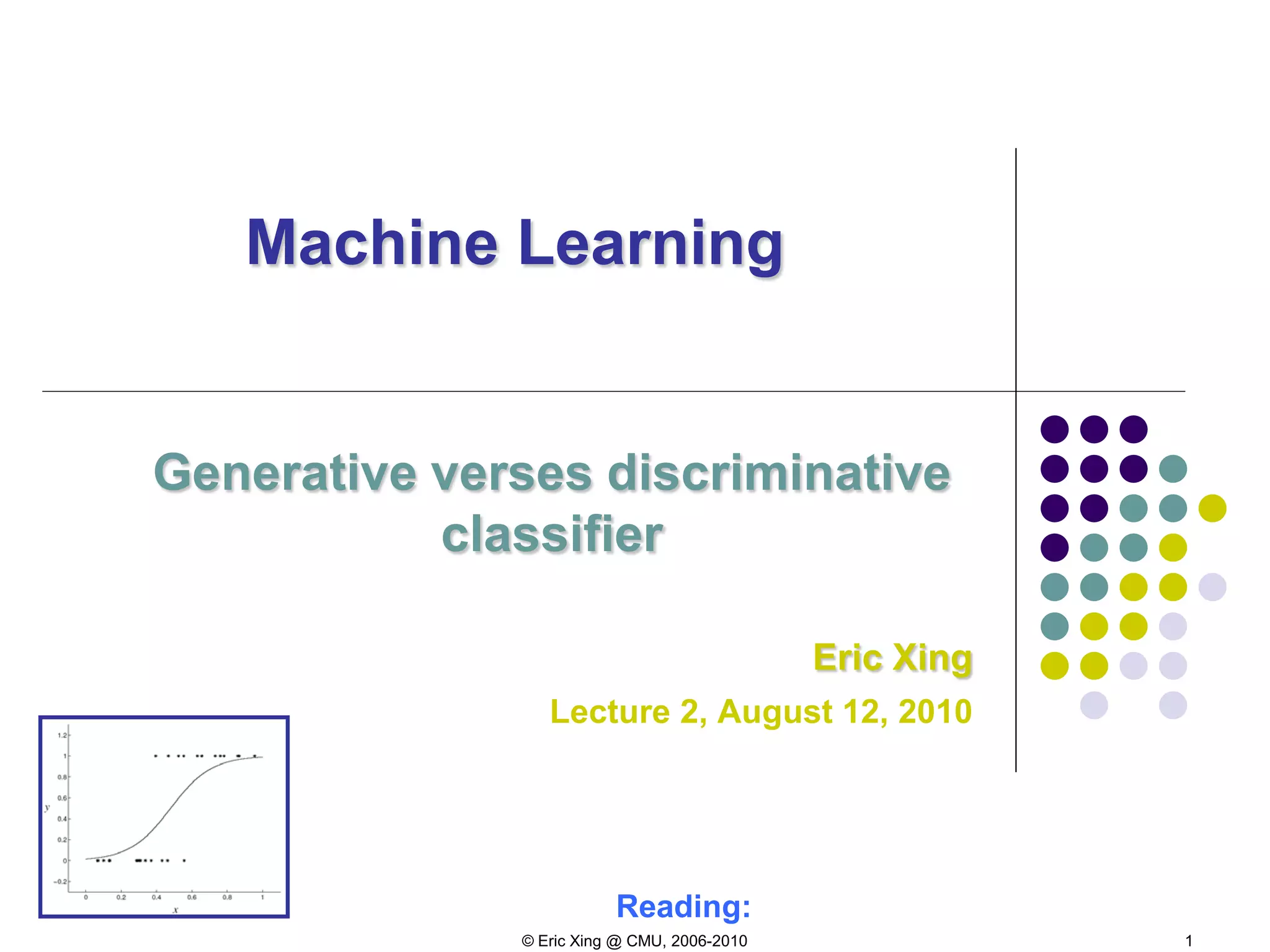
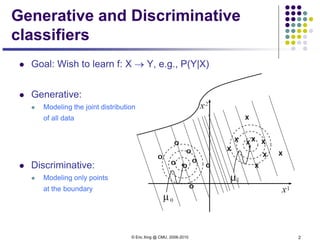
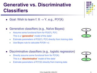
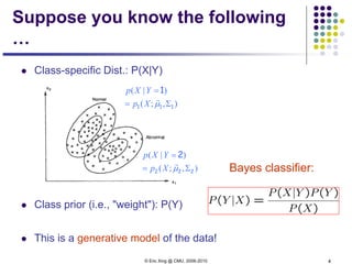
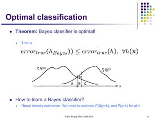
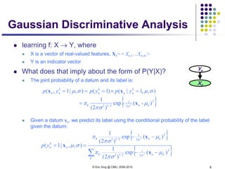
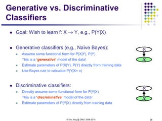
Generative and Discriminative
classifiers
 Goal: Wish to learn f: X → Y, e.g., P(Y|X)
 Generative:
 Modeling the joint distribution
of all data
 Discriminative:
 Modeling only points
at the boundary

3. © Eric Xing @ CMU, 2006-2010 3
Generative vs. Discriminative
Classifiers
 Goal: Wish to learn f: X → Y, e.g., P(Y|X)
 Generative classifiers (e.g., Naïve Bayes):
 Assume some functional form for P(X|Y), P(Y)
This is a ‘generative’ model of the data!
 Estimate parameters of P(X|Y), P(Y) directly from training data
 Use Bayes rule to calculate P(Y|X= x)
 Discriminative classifiers (e.g., logistic regression)
 Directly assume some functional form for P(Y|X)
This is a ‘discriminative’ model of the data!
 Estimate parameters of P(Y|X) directly from training data
Yn
Xn
Yn
Xn

4. © Eric Xing @ CMU, 2006-2010 4
Suppose you know the following
…
 Class-specific Dist.: P(X|Y)
 Class prior (i.e., "weight"): P(Y)
 This is a generative model of the data!
),;(
)|(
111
1
Σ=
=
µ

Xp
YXp
),;(
)|(
222
2
Σ=
=
µ

Xp
YXp
Bayes classifier:

5. © Eric Xing @ CMU, 2006-2010 5
Optimal classification
 Theorem: Bayes classifier is optimal!
 That is
 How to learn a Bayes classifier?
 Recall density estimation. We need to estimate P(X|y=k), and P(y=k) for all k

6. © Eric Xing @ CMU, 2006-2010 6
Gaussian Discriminative Analysis
 learning f: X → Y, where
 X is a vector of real-valued features, Xn= < Xn,1…Xn,m >
 Y is an indicator vector
 What does that imply about the form of P(Y|X)?
 The joint probability of a datum and its label is:
 Given a datum xn, we predict its label using the conditional probability of the label
given the datum:
Yn
Xn
{ }2
2
1
2/12
)-(-exp
)2(
1
),,1|()1(),|1,(
2 knk
k
nn
k
n
k
nn ypypyp
µ
πσ
π
σµσµ
σ
x
xx
=
=×===
{ }
{ }∑ −−
−−
==
'
2
'2
1
2/12'
2
2
1
2/12
)(exp
)2(
1
)(exp
)2(
1
),,|1(
2
2
k
knk
knk
n
k
nyp
µ
πσ
π
µ
πσ
π
σµ
σ
σ
x
x
x

7. © Eric Xing @ CMU, 2006-2010 7
Conditional Independence
 X is conditionally independent of Y given Z, if the probability
distribution governing X is independent of the value of Y, given
the value of Z
Which we often write
 e.g.,
 Equivalent to:

8. © Eric Xing @ CMU, 2006-2010 8
Naïve Bayes Classifier
 When X is multivariate-Gaussian vector:
 The joint probability of a datum and it label is:
 The naïve Bayes simplification
 More generally:
 Where p(. | .) is an arbitrary conditional (discrete or continuous) 1-D density
{ })-()-(-exp
)2(
1
),,1|()1(),|1,(
1
2
1
2/1 kn
T
knk
k
nn
k
n
k
nn ypypyp
µµ
π
π
µµ


xx
xx
−
Σ
Σ
=
Σ=×==Σ=
Yn
Xn
{ }∏
∏
=
=×===
j
jkjn
jk
k
j
jkjk
k
njn
k
n
k
nn
x
yxpypyp
jk
2
,,2
1
2/12
,
,,,
)-(-exp
)2(
1
),,1|()1(),|1,(
2
,
µ
πσ
π
σµσµ
σ
x
∏=
×=
m
j
njnnnn yxpypyp
1
, ),|()|(),|,( ηππηx
Yn
Xn,1 Xn,2 Xn,m
…

9. © Eric Xing @ CMU, 2006-2010 9
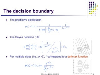
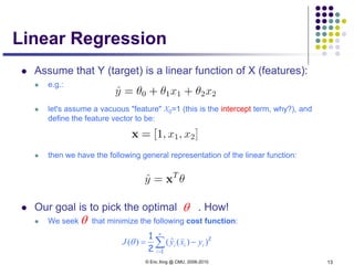
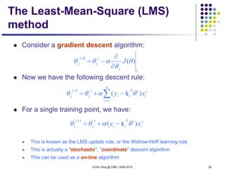
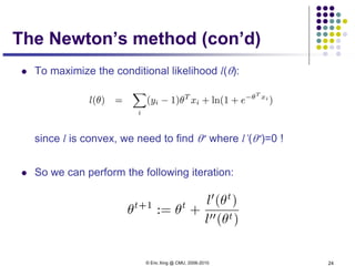
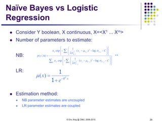
The predictive distribution
 Understanding the predictive distribution
 Under naïve Bayes assumption:
 For two class (i.e., K=2), and when the two classes haves the same
variance, ** turns out to be a logistic function
*
),|,(
),|,(
),|(
),,|,(
),,,|(
' '''∑ Σ
Σ
=
Σ
Σ=
=Σ=
k kknk
kknk
n
n
k
n
n
k
n
xN
xN
xp
xyp
xyp
µπ
µπ
µ
πµ
πµ 

 1
1
( ){ }1
1
222
122
1
1
2
222
1
2
12
21
1
21
1
1
1
1
1
π
π
σσσµπ
σµπ
µµµµ
σ
σ
)(2
log)-(exp
log)-(exp
log)][-]([)-(exp −
















−−−
















−−−
++−+
=
∑
∑
+
=
∑j
jjjjj
nCx
Cx
jj
j j
jj
n
j
j j
jj
n
j
x
n
T
x
e θ−
+
=
1
1
)|( nn xyp 11
=
**
log)(exp
log)(exp
),,,|(
' ,''
,'
'
,
,
∑ ∑
∑
















−−−−
















−−−−
=Σ=
k j jk
j
k
j
n
jk
k
j jk
j
k
j
n
jk
k
n
k
n
Cx
Cx
xyp
σµ
σ
π
σµ
σ
π
πµ
2
2
2
2
2
1
2
1
1


10. © Eric Xing @ CMU, 2006-2010 10
The decision boundary
 The predictive distribution
 The Bayes decision rule:
 For multiple class (i.e., K>2), * correspond to a softmax function
∑
−
−
==
j
x
x
n
k
n
n
T
j
n
T
k
e
e
xyp θ
θ
)|( 1
n
T
xM
j
j
nj
nn
e
x
xyp θ
θθ
−
=
+
=






−−+
==
∑
1
1
1
1
1
0
1
1
exp
)|(
n
T
x
x
x
nn
nn
x
e
e
e
xyp
xyp
n
T
n
T
n
T
θ
θ
θ
θ
=












+
+=
=
=
−
−
−
1
1
1
1
1
2
1
ln
)|(
)|(
ln

11. © Eric Xing @ CMU, 2006-2010 11
Generative vs. Discriminative
Classifiers
 Goal: Wish to learn f: X → Y, e.g., P(Y|X)
 Generative classifiers (e.g., Naïve Bayes):
 Assume some functional form for P(X|Y), P(Y)
This is a ‘generative’ model of the data!
 Estimate parameters of P(X|Y), P(Y) directly from training data
 Use Bayes rule to calculate P(Y|X= x)
 Discriminative classifiers:
 Directly assume some functional form for P(Y|X)
This is a ‘discriminative’ model of the data!
 Estimate parameters of P(Y|X) directly from training data
Yi
Xi
Yi
Xi

12. © Eric Xing @ CMU, 2006-2010 12
Linear Regression
 The data:
 Both nodes are observed:
 X is an input vector
 Y is a response vector
(we first consider y as a generic
continuous response vector, then
we consider the special case of
classification where y is a discrete
indicator)
 A regression scheme can be
used to model p(y|x) directly,
rather than p(x,y)
Yi
Xi
N
{ }),(,),,(),,(),,( NN yxyxyxyx 332211

13. © Eric Xing @ CMU, 2006-2010 13
Linear Regression
 Assume that Y (target) is a linear function of X (features):
 e.g.:
 let's assume a vacuous "feature" X0=1 (this is the intercept term, why?), and
define the feature vector to be:
 then we have the following general representation of the linear function:
 Our goal is to pick the optimal . How!
 We seek that minimize the following cost function:
θ
θ
∑=
−=
n
i
iii yxyJ
1
2
2
1
))(ˆ()(

θ

14. © Eric Xing @ CMU, 2006-2010 14
The Least-Mean-Square (LMS)
method
 Consider a gradient descent algorithm:
 Now we have the following descent rule:
 For a single training point, we have:
 This is known as the LMS update rule, or the Widrow-Hoff learning rule
 This is actually a "stochastic", "coordinate" descent algorithm
 This can be used as a on-line algorithm
∑=
+
−+=
n
i
j
i
tT
ii
t
j
t
j xy
1
1
)( θαθθ x

j
i
tT
ii
t
j
t
j xy )(
1
θαθθ x

−+=
+
tj
t
j
t
j J )(θ
θ
αθθ
∂
∂
−=
+1

15. © Eric Xing @ CMU, 2006-2010 15
Probabilistic Interpretation of
LMS
 Let us assume that the target variable and the inputs are
related by the equation:
where ε is an error term of unmodeled effects or random noise
 Now assume that ε follows a Gaussian N(0,σ), then we have:
 By independence assumption:
ii
T
iy εθ += x





 −
−= 2
2
22
1
σ
θ
σπ
θ
)(
exp);|( i
T
i
ii
y
xyp
x







 −
−





==
∑
∏ =
=
2
1
2
1 22
1
σ
θ
σπ
θθ
n
i i
T
i
nn
i
ii
y
xypL
)(
exp);|()(
x

16. © Eric Xing @ CMU, 2006-2010 16
Probabilistic Interpretation of
LMS, cont.
 Hence the log-likelihood is:
 Do you recognize the last term?
Yes it is:
 Thus under independence assumption, LMS is equivalent to
MLE of θ !
∑=
−−=
n
i i
T
iynl 1
2
2
2
11
2
1
)(log)( xθ
σσπ
θ
∑=
−=
n
i
i
T
i yJ
1
2
2
1
)()( θθ x

17. © Eric Xing @ CMU, 2006-2010 17
Classification and logistic
regression

18. © Eric Xing @ CMU, 2006-2010 18
The logistic function

19. © Eric Xing @ CMU, 2006-2010 19
Logistic regression (sigmoid
classifier)
 The condition distribution: a Bernoulli
where µ is a logistic function
 We can used the brute-force gradient method as in LR
 But we can also apply generic laws by observing the p(y|x) is
an exponential family function, more specifically, a
generalized linear model (see future lectures …)
yy
xxxyp −
−= 1
1 ))(()()|( µµ
xT
e
x θ
µ −
+
=
1
1
)(

20. © Eric Xing @ CMU, 2006-2010 20
Training Logistic Regression:
MCLE
 Estimate parameters θ=<θ0, θ1, ... θm> to maximize the
conditional likelihood of training data
 Training data
 Data likelihood =
 Data conditional likelihood =

21. © Eric Xing @ CMU, 2006-2010 21
Expressing Conditional Log
Likelihood
 Recall the logistic function:
and conditional likelihood:

22. © Eric Xing @ CMU, 2006-2010 22
Maximizing Conditional Log
Likelihood
 The objective:
 Good news: l(θ) is concave function of θ
 Bad news: no closed-form solution to maximize l(θ)

23. © Eric Xing @ CMU, 2006-2010 23
The Newton’s method
 Finding a zero of a function

24. © Eric Xing @ CMU, 2006-2010 24
The Newton’s method (con’d)
 To maximize the conditional likelihood l(θ):
since l is convex, we need to find θ∗ where l’(θ∗)=0 !
 So we can perform the following iteration:

25. © Eric Xing @ CMU, 2006-2010 25
The Newton-Raphson method
 In LR the θ is vector-valued, thus we need the following
generalization:
 ∇ is the gradient operator over the function
 H is known as the Hessian of the function

26. © Eric Xing @ CMU, 2006-2010 26
The Newton-Raphson method
 In LR the θ is vector-valued, thus we need the following
generalization:
 ∇ is the gradient operator over the function
 H is known as the Hessian of the function

27. © Eric Xing @ CMU, 2006-2010 27
Iterative reweighed least squares
(IRLS)
 Recall in the least square est. in linear regression, we have:
which can also derived from Newton-Raphson
 Now for logistic regression:

28. © Eric Xing @ CMU, 2006-2010 28
Generative vs. Discriminative
Classifiers
 Goal: Wish to learn f: X → Y, e.g., P(Y|X)
 Generative classifiers (e.g., Naïve Bayes):
 Assume some functional form for P(X|Y), P(Y)
This is a ‘generative’ model of the data!
 Estimate parameters of P(X|Y), P(Y) directly from training data
 Use Bayes rule to calculate P(Y|X= x)
 Discriminative classifiers:
 Directly assume some functional form for P(Y|X)
This is a ‘discriminative’ model of the data!
 Estimate parameters of P(Y|X) directly from training data
Yi
Xi
Yi
Xi

29. © Eric Xing @ CMU, 2006-2010 29
Naïve Bayes vs Logistic
Regression
 Consider Y boolean, X continuous, X=<X1 ... Xm>
 Number of parameters to estimate:
NB:
LR:
 Estimation method:
 NB parameter estimates are uncoupled
 LR parameter estimates are coupled
**
log)(
2
1
exp
log)(
2
1
exp
)|(
' ,'
2
,'2
,'
'
,
2
,2
,
∑ ∑
∑
















−−−−
















−−−−
=
k j jkjkj
jk
k
j jkjkj
jk
k
Cx
Cx
yp
σµ
σ
π
σµ
σ
π
x
xT
e
x θ
µ −
+
=
1
1
)(

30. © Eric Xing @ CMU, 2006-2010 30
Naïve Bayes vs Logistic
Regression
 Asymptotic comparison (# training examples → infinity)
 when model assumptions correct
 NB, LR produce identical classifiers
 when model assumptions incorrect
 LR is less biased – does not assume conditional independence
 therefore expected to outperform NB

31. © Eric Xing @ CMU, 2006-2010 31
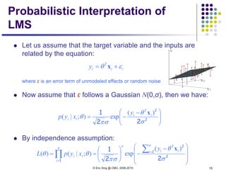
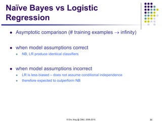
Naïve Bayes vs Logistic
Regression
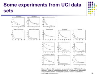
 Non-asymptotic analysis (see [Ng & Jordan, 2002] )
 convergence rate of parameter estimates – how many training
examples needed to assure good estimates?
NB order log m (where m = # of attributes in X)
LR order m
 NB converges more quickly to its (perhaps less helpful)
asymptotic estimates

32. © Eric Xing @ CMU, 2006-2010 32
Some experiments from UCI data
sets

33. © Eric Xing @ CMU, 2006-2010 33
Robustness
• The best fit from a quadratic
regression
• But this is probably better …

34. © Eric Xing @ CMU, 2006-2010 34
Bayesian Parameter Estimation
 Treat the distribution parameters θ also as a random variable
 The a posteriori distribution of θ after seem the data is:
This is Bayes Rule
likelihoodmarginal
priorlikelihood
posterior
×
=
∫
==
θθθ
θθθθ
θ
dpDp
pDp
Dp
pDp
Dp
)()|(
)()|(
)(
)()|(
)|(
The prior p(.) encodes our prior knowledge about the domain

35. © Eric Xing @ CMU, 2006-2010 35
35
What if is not invertible ?
log likelihood log prior
Prior belief that β is Gaussian with zero-mean biases solution to “small” β
I) Gaussian Prior
0
Ridge Regression
Closed form: HW
Regularized Least Squares and
MAP

36. © Eric Xing @ CMU, 2006-2010 36
Regularized Least Squares and
MAP
36
What if is not invertible ?
log likelihood log prior
Prior belief that β is Laplace with zero-mean biases solution to “small” β
Lasso
Closed form: HW
II) Laplace Prior

37. © Eric Xing @ CMU, 2006-2010 37
Ridge Regression vs Lasso
37
Ridge Regression: Lasso: HOT
!
Lasso (l1 penalty) results in sparse solutions – vector with more zero coordinates
Good for high-dimensional problems – don’t have to store all coordinates!
βs with
constant
l1 norm
βs with constant J(β)
(level sets of J(β))
βs with
constant
l2 norm
β2
β1

38. © Eric Xing @ CMU, 2006-2010 38
Case study:
predicting gene expression
The genetic picture
CGTTTCACTGTACAATTT
causal SNPs
a univariate phenotype:
i.e., the expression intensity of
a gene

39. © Eric Xing @ CMU, 2006-2010 39
Individual 1
Individual 2
Individual N
Phenotype (BMI)
2.5
4.8
4.7
Genotype
. . C . . . . . T . . C . . . . . . . T . . .
. . C . . . . . A . . C . . . . . . . T . . .
. . G . . . . . A . . G . . . . . . . A . . .
. . C . . . . . T . . C . . . . . . . T . . .
. . G . . . . . T . . C . . . . . . . T . . .
. . G . . . . . T . . G . . . . . . . T . . .
Causal SNPBenign SNPs
…
Association Mapping as
Regression

40. © Eric Xing @ CMU, 2006-2010 40
Individual 1
Individual 2
Individual N
Phenotype (BMI)
2.5
4.8
4.7
Genotype
. . 0 . . . . . 1 . . 0 . . . . . . . 0 . . .
. . 1 . . . . . 1 . . 1 . . . . . . . 1 . . .
. . 2 . . . . . 2 . . 1 . . . . . . . 0 . . .
…
yi = ∑=
J
j
jijx
1
β SNPs with large
|βj| are relevant
Association Mapping as
Regression

41. © Eric Xing @ CMU, 2006-2010 41
Experimental setup
 Asthama dataset
 543 individuals, genotyped at 34 SNPs
 Diploid data was transformed into 0/1 (for homozygotes) or 2 (for heterozygotes)
 X=543x34 matrix
 Y=Phenotype variable (continuous)
 A single phenotype was used for regression
 Implementation details
 Iterative methods: Batch update and online update implemented.
 For both methods, step size α is chosen to be a small fixed value (10-6). This
choice is based on the data used for experiments.
 Both methods are only run to a maximum of 2000 epochs or until the change in
training MSE is less than 10-4

42. © Eric Xing @ CMU, 2006-2010 42© Eric Xing @ CMU, 2006-2008 42
 For the batch method, the training MSE is initially large due to uninformed initialization
 In the online update, N updates for every epoch reduces MSE to a much smaller value.
Convergence Curves

43. © Eric Xing @ CMU, 2006-2010 43
The Learned Coefficients

44. © Eric Xing @ CMU, 2006-2010 44
 The results from B and O
update are almost identical.
So the plots coincide.
 The test MSE from the
normal equation is more
than that of B and O during
small training. This is
probably due to overfitting.
 In B and O, since only 2000
iterations are allowed at
most. This roughly acts as a
mechanism that avoids
overfitting.
Performance vs. Training Size

45. © Eric Xing @ CMU, 2006-2010 45
Summary
 Naïve Bayes classifier
 What’s the assumption
 Why we use it
 How do we learn it
 Logistic regression
 Functional form follows from Naïve Bayes assumptions
 For Gaussian Naïve Bayes assuming variance
 For discrete-valued Naïve Bayes too
 But training procedure picks parameters without the conditional independence
assumption
 Gradient ascent/descent
 – General approach when closed-form solutions unavailable
 Generative vs. Discriminative classifiers
 – Bias vs. variance tradeoff

46. © Eric Xing @ CMU, 2006-2010 46
Appendix

47. © Eric Xing @ CMU, 2006-2010 47
Parameter Learning from iid Data
 Goal: estimate distribution parameters θ from a dataset of N
independent, identically distributed (iid), fully observed,
training cases
D = {x1, . . . , xN}
 Maximum likelihood estimation (MLE)
1. One of the most common estimators
2. With iid and full-observability assumption, write L(θ) as the likelihood of the data:
3. pick the setting of parameters most likely to have generated the data we saw:
);,,()( , θθ NxxxPL 21=
∏=
=
=
N
i i
N
xP
xPxPxP
1
2
);(
);(,),;();(
θ
θθθ 
)(maxarg*
θθ
θ
L= )(logmaxarg θ
θ
L=

48. © Eric Xing @ CMU, 2006-2010 48
Example: Bernoulli model
 Data:
 We observed N iid coin tossing: D={1, 0, 1, …, 0}
 Representation:
Binary r.v:
 Model:
 How to write the likelihood of a single observation xi ?
 The likelihood of datasetD={x1, …,xN}:
ii xx
ixP −
−= 1
1 )()( θθ
( )∏∏ =
−
=
−==
N
i
xx
N
i
iN
ii
xPxxxP
1
1
1
21 1 )()|()|,...,,( θθθθ
},{ 10=nx
tails#head#
)()( θθθθ −=
∑
−
∑
= ==
−
11 11
1
N
i
i
N
i
i xx



=
=−
=
1
01
x
x
xP
for
for
)(
θ
θ xx
xP −
−= 1
1 )()( θθ⇒

49. © Eric Xing @ CMU, 2006-2010 49
Maximum Likelihood Estimation
 Objective function:
 We need to maximize this w.r.t. θ
 Take derivatives wrt θ
 Sufficient statistics
 The counts, are sufficient statistics of data D
)log()(log)(log)|(log);( θθθθθθ −−+=−== 11 hh
nn
nNnDPD th
l
0
1
=
−
−
−=
∂
∂
θθθ
hh nNnl
N
nh
MLE =θ

∑=
i
iMLE x
N
1
θ

or
Frequency as
sample mean
,where, ∑= i ikh xnn

50. © Eric Xing @ CMU, 2006-2010 50
Overfitting
 Recall that for Bernoulli Distribution, we have
 What if we tossed too few times so that we saw zero head?
We have and we will predict that the probability of
seeing a head next is zero!!!
 The rescue: "smoothing"
 Where n' is know as the pseudo- (imaginary) count
 But can we make this more formal?
tailhead
head
head
ML
nn
n
+
=θ

,0=head
MLθ

'
'
nnn
nn
tailhead
head
head
ML
++
+
=θ


51. © Eric Xing @ CMU, 2006-2010 51
Bayesian Parameter Estimation
 Treat the distribution parameters θ also as a random variable
 The a posteriori distribution of θ after seem the data is:
This is Bayes Rule
likelihoodmarginal
priorlikelihood
posterior
×
=
∫
==
θθθ
θθθθ
θ
dpDp
pDp
Dp
pDp
Dp
)()|(
)()|(
)(
)()|(
)|(
The prior p(.) encodes our prior knowledge about the domain

52. © Eric Xing @ CMU, 2006-2010 52
Frequentist Parameter Estimation
Two people with different priors p(θ) will end up with
different estimates p(θ|D).
 Frequentists dislike this “subjectivity”.
 Frequentists think of the parameter as a fixed, unknown
constant, not a random variable.
 Hence they have to come up with different "objective"
estimators (ways of computing from data), instead of using
Bayes’ rule.
 These estimators have different properties, such as being “unbiased”, “minimum
variance”, etc.
 The maximum likelihood estimator, is one such estimator.

53. © Eric Xing @ CMU, 2006-2010 53
Discussion
θ or p(θ), this is the problem!
Bayesians know it

54. © Eric Xing @ CMU, 2006-2010 54
Bayesian estimation for Bernoulli
 Beta distribution:
 When x is discrete
 Posterior distribution of θ :
 Notice the isomorphism of the posterior to the prior,
 such a prior is called a conjugate prior
 α and β are hyperparameters (parameters of the prior) and correspond to the
number of “virtual” heads/tails (pseudo counts)
1111
1
1
1 111 −+−+−−
−=−×−∝= βαβα
θθθθθθ
θθ
θ thth nnnn
N
N
N
xxp
pxxp
xxP )()()(
),...,(
)()|,...,(
),...,|(
1111
11 −−−−
−=−
ΓΓ
+Γ
= βαβα
θθβαθθ
βα
βα
βαθ )(),()(
)()(
)(
),;( BP
!)()( xxxx =Γ=+Γ 1

55. © Eric Xing @ CMU, 2006-2010 55
Bayesian estimation for
Bernoulli, con'd
 Posterior distribution of θ :
 Maximum a posteriori (MAP) estimation:
 Posterior mean estimation:
 Prior strength: A=α+β
 A can be interoperated as the size of an imaginary data set from which we obtain
the pseudo-counts
1111
1
1
1 111 −+−+−−
−=−×−∝= βαβα
θθθθθθ
θθ
θ thth nnnn
N
N
N
xxp
pxxp
xxP )()()(
),...,(
)()|,...,(
),...,|(
∫ ∫ ++
+
=−×== −+−+
βα
α
θθθθθθθθ βα
N
n
dCdDp hnn
Bayes
th 11
1 )()|(
Bata parameters
can be understood
as pseudo-counts
),...,|(logmaxarg NMAP xxP 1θθ
θ
=

56. © Eric Xing @ CMU, 2006-2010 56
Effect of Prior Strength
 Suppose we have a uniform prior (α=β=1/2),
and we observe
 Weak prior A = 2. Posterior prediction:
 Strong prior A = 20. Posterior prediction:
 However, if we have enough data, it washes away the prior.
e.g., . Then the estimates under
weak and strong prior are and , respectively,
both of which are close to 0.2
),( 82 === th nnn

250
102
21
282 .)',,|( =
+
+
=×==== αα

th nnhxp
400
1020
210
2082 .)',,|( =
+
+
=×==== αα

th nnhxp
),( 800200 === th nnn

10002
2001
+
+
100020
20010
+
+

57. © Eric Xing @ CMU, 2006-2010 57
Example 2: Gaussian density
 Data:
 We observed N iid real samples:
D={-0.1, 10, 1, -5.2, …, 3}
 Model:
 Log likelihood:
 MLE: take derivative and set to zero:
( ) { }22212
22 σµπσ /)(exp)(
/
−−=
−
xxP
( )
∑=
−
−−==
N
n
nxN
DPD
1
2
2
2
2
1
2
2 σ
µ
πσθθ )log()|(log);(l
( )
( )∑
∑
−+−=
∂
∂
−=
∂
∂
n n
n n
x
N
x
2
422
2
2
1
2
1
µ
σσσ
µσ
µ
l
l
)/( ( )
( )∑
∑
−=
=
n MLnMLE
n nMLE
x
N
x
N
22 1
1
µσ
µ

58. © Eric Xing @ CMU, 2006-2010 58
MLE for a multivariate-Gaussian
 It can be shown that the MLE for µ and Σ is
where the scatter matrix is
 The sufficient statistics are Σnxn and Σnxnxn
T.
 Note that XTX=Σnxnxn
T may not be full rank (eg. if N <D), in which case ΣML is not
invertible
( )
( )( ) S
N
xx
N
x
N
n
T
MLnMLnMLE
n nMLE
11
1
=−−=Σ
=
∑
∑
µµ
µ
( )( ) ( ) T
MLMLn n
T
nnn
T
MLnMLn NxxxxS µµµµ −=−−= ∑∑














=
K
n
n
n
n
x
x
x
x

2
1














−−−−−−
−−−−−−
−−−−−−
=
T
N
T
T
x
x
x
X

2
1

59. © Eric Xing @ CMU, 2006-2010 59
Bayesian estimation
 Normal Prior:
 Joint probability:
 Posterior:
( ) { }2
0
2
0
212
0 22 σµµπσµ /)(exp)(
/
−−=
−
P
1
2
0
2
2
02
0
2
2
0
2
0
2
2
1
1
1
1
−






+=
+
+
+
=
σσ
σµ
σσ
σ
σσ
σ
µ
N
N
x
N
N ~and,
//
/
//
/~where
Sample mean
( ) ( )
( ) { }2
0
2
0
212
0
1
2
2
22
22
2
1
2
σµµπσ
µ
σ
πσµ
/)(exp
exp),(
/
/
−−×






−−=
−
=
−
∑
N
n
n
N
xxP
( ) { }22212
22 σµµσπµ ~/)~(exp~)|(
/
−−=
−
xP

60. © Eric Xing @ CMU, 2006-2010 60
Bayesian estimation: unknown µ, known σ
 The posterior mean is a convex combination of the prior and the MLE, with
weights proportional to the relative noise levels.
 The precision of the posterior 1/σ2
N is the precision of the prior 1/σ2
0 plus one
contribution of data precision 1/σ2 for each observed data point.
 Sequentially updating the mean
 µ∗ = 0.8 (unknown), (σ2)∗ = 0.1 (known)
 Effect of single data point
 Uninformative (vague/ flat) prior, σ2
0 →∞
1
2
0
2
2
02
0
2
2
0
2
0
2
2
1
1
1
1
−






+=
+
+
+
=
σσ
σµ
σσ
σ
σσ
σ
µ
N
N
x
N
N
N
~,
//
/
//
/
2
0
2
2
0
02
0
2
2
0
001
σσ
σ
µ
σσ
σ
µµµ
+
−−=
+
−+= )()( xxx
0µµ →N