Download as PDF, PPTX


![Posterior distribution
Central concept of Bayesian inference:
π( θ
parameter
| xobs
observation
) ∝ π(θ)
prior
× L(θ | xobs
)
likelihood
Drives
derivation of optimal decisions
assessment of uncertainty
model selection
[McElreath, 2015]](https://image.slidesharecdn.com/jsm19-190720162758/75/the-ABC-of-ABC-5-2048.jpg)
![Monte Carlo representation
Exploration of posterior π(θ|xobs) may require to produce
sample
θ1, . . . , θT
distributed from π(θ|xobs) (or asymptotically by Markov chain
Monte Carlo)
[McElreath, 2015]](https://image.slidesharecdn.com/jsm19-190720162758/75/the-ABC-of-ABC-6-2048.jpg)

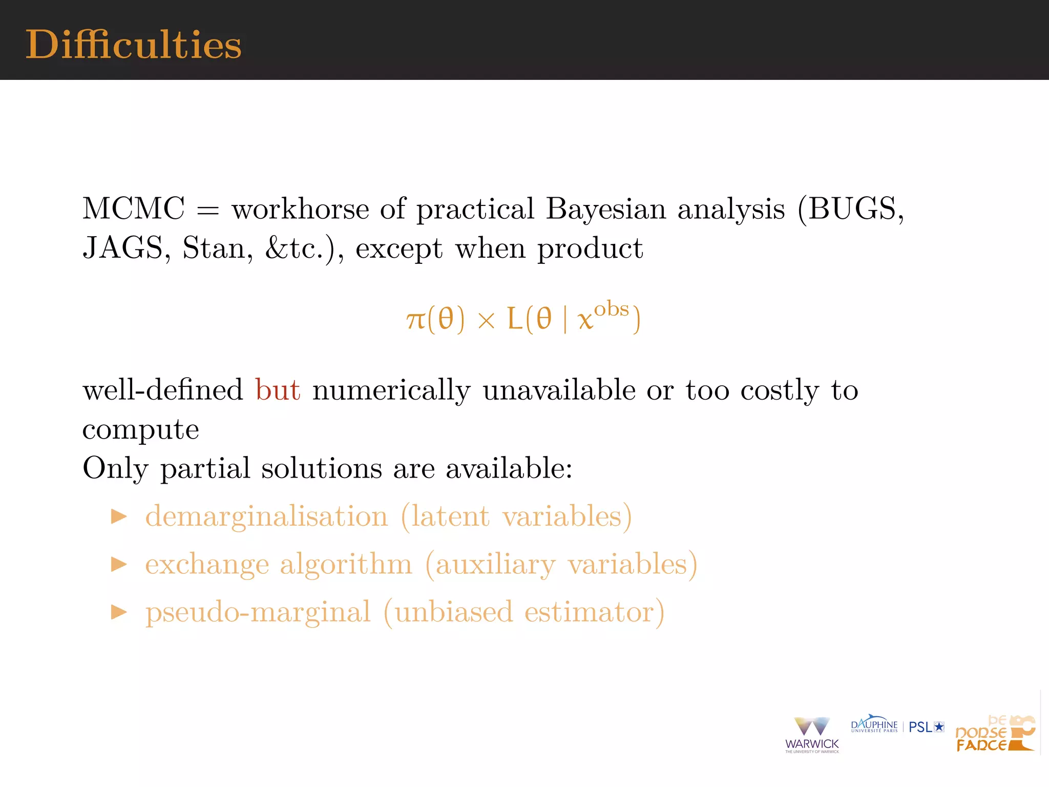
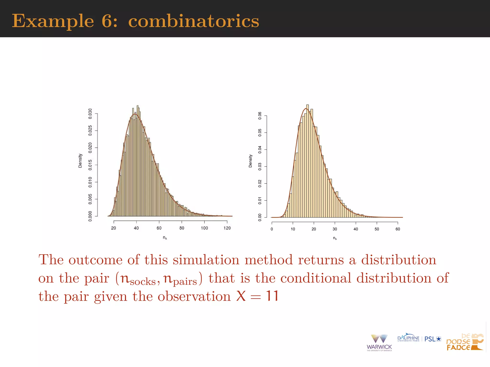
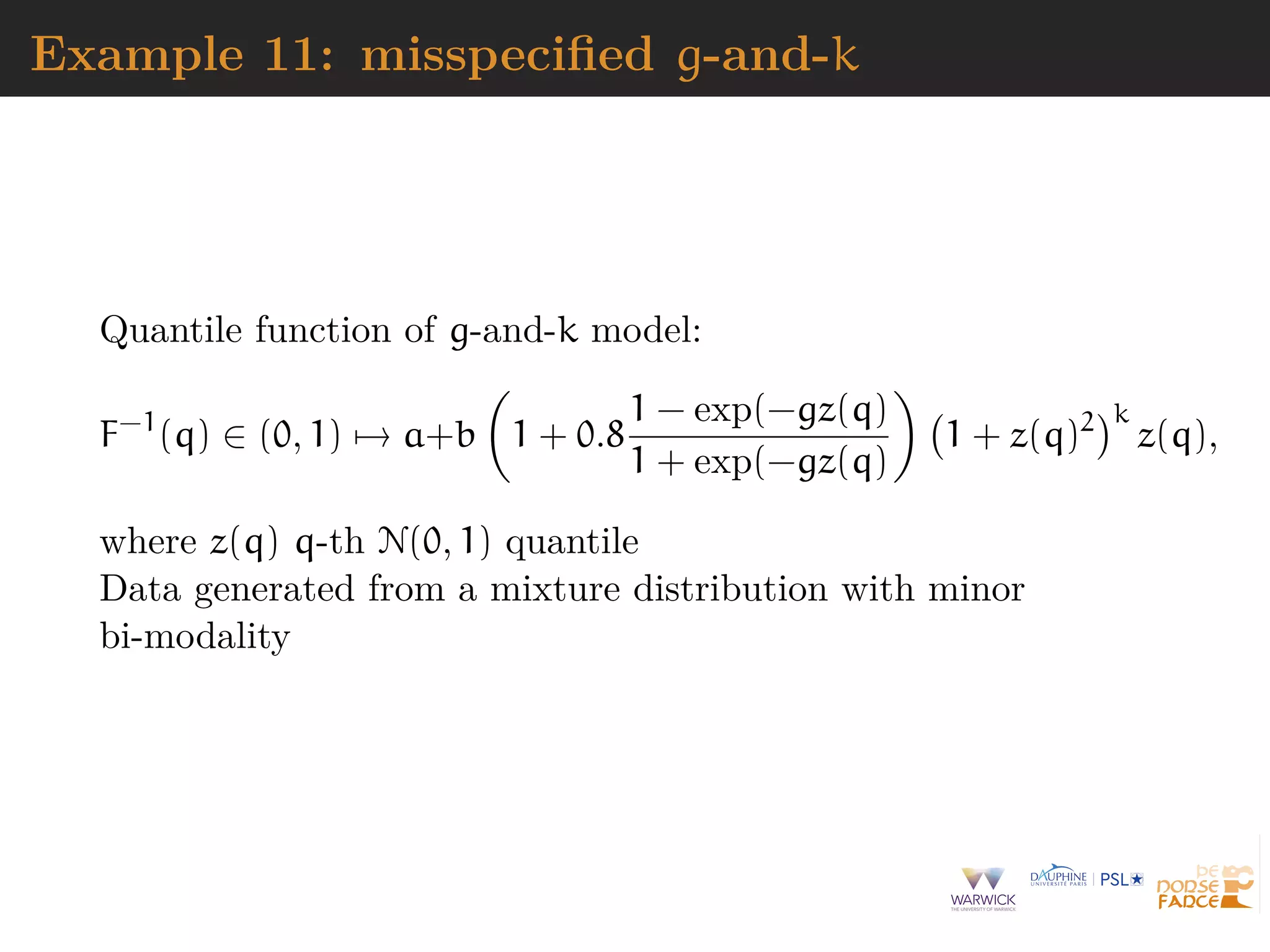
![Example 1: Dynamic mixture
Mixture model
{1 − wµ,τ(x)}fβ,λ(x) + wµ,τ(x)gε,σ(x) x > 0
where fβ,λ Weibull density, gε,σ generalised Pareto density, and
wµ,τ Cauchy cdf
Intractable normalising constant
C(µ, τ, β, λ, ε, σ) =
∞
0
{(1 − wµ,τ(x))fβ,λ(x) + wµ,τ(x)gε,σ(x)} dx
[Frigessi, Haug & Rue, 2002]](https://image.slidesharecdn.com/jsm19-190720162758/75/the-ABC-of-ABC-9-2048.jpg)
![Example 5: exponential random graph
ERGM: binary random vector x indexed
by all edges on set of nodes plus graph
f(x | θ) =
1
C(θ)
exp(θT
S(x))
with S(x) vector of statistics and C(θ)
intractable normalising constant
[Grelaud & al., 2009; Everitt, 2012; Bouranis & al., 2017]](https://image.slidesharecdn.com/jsm19-190720162758/75/the-ABC-of-ABC-13-2048.jpg)
![A?B?C?
A stands for approximate [wrong
likelihood]
B stands for Bayesian [right prior]
C stands for computation [producing
a parameter sample]](https://image.slidesharecdn.com/jsm19-190720162758/75/the-ABC-of-ABC-15-2048.jpg)
![A?B?C?
Rough version of the data [from dot
to ball]
Non-parametric approximation of
the likelihood [near actual
observation]
Use of non-sufficient statistics
[dimension reduction]
Monte Carlo error [and no
unbiasedness]](https://image.slidesharecdn.com/jsm19-190720162758/75/the-ABC-of-ABC-16-2048.jpg)
![A?B?C?
“Marin et al. (2012) proposed
Approximate Bayesian Computation
(ABC), which is more complex than
MCMC, but outputs cruder estimates”
[Heavens et al., 2017]](https://image.slidesharecdn.com/jsm19-190720162758/75/the-ABC-of-ABC-17-2048.jpg)
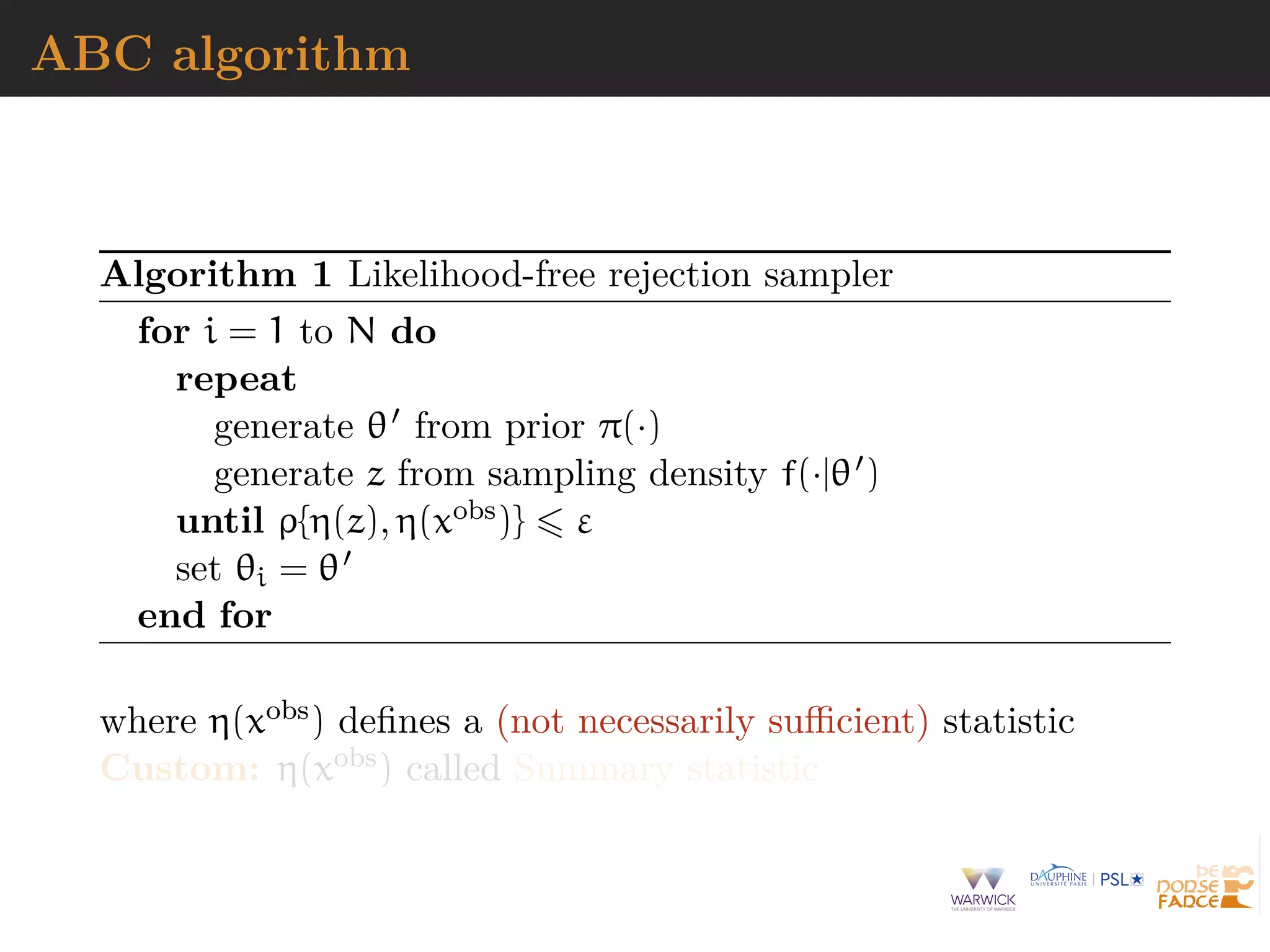
![A seemingly na¨ıve representation
When likelihood f(x|θ) not in closed form, likelihood-free
rejection technique:
ABC algorithm
For an observation xobs ∼ f(x|θ), under the prior π(θ), keep
jointly simulating
θ ∼ π(θ) , z ∼ f(z|θ ) ,
until the auxiliary variable z is equal to the observed value,
z = xobs
[Diggle & Gratton, 1984; Rubin, 1984; Tavar´e et al., 1997]](https://image.slidesharecdn.com/jsm19-190720162758/75/the-ABC-of-ABC-18-2048.jpg)
![A seemingly na¨ıve representation
When likelihood f(x|θ) not in closed form, likelihood-free
rejection technique:
ABC algorithm
For an observation xobs ∼ f(x|θ), under the prior π(θ), keep
jointly simulating
θ ∼ π(θ) , z ∼ f(z|θ ) ,
until the auxiliary variable z is equal to the observed value,
z = xobs
[Diggle & Gratton, 1984; Rubin, 1984; Tavar´e et al., 1997]](https://image.slidesharecdn.com/jsm19-190720162758/75/the-ABC-of-ABC-19-2048.jpg)
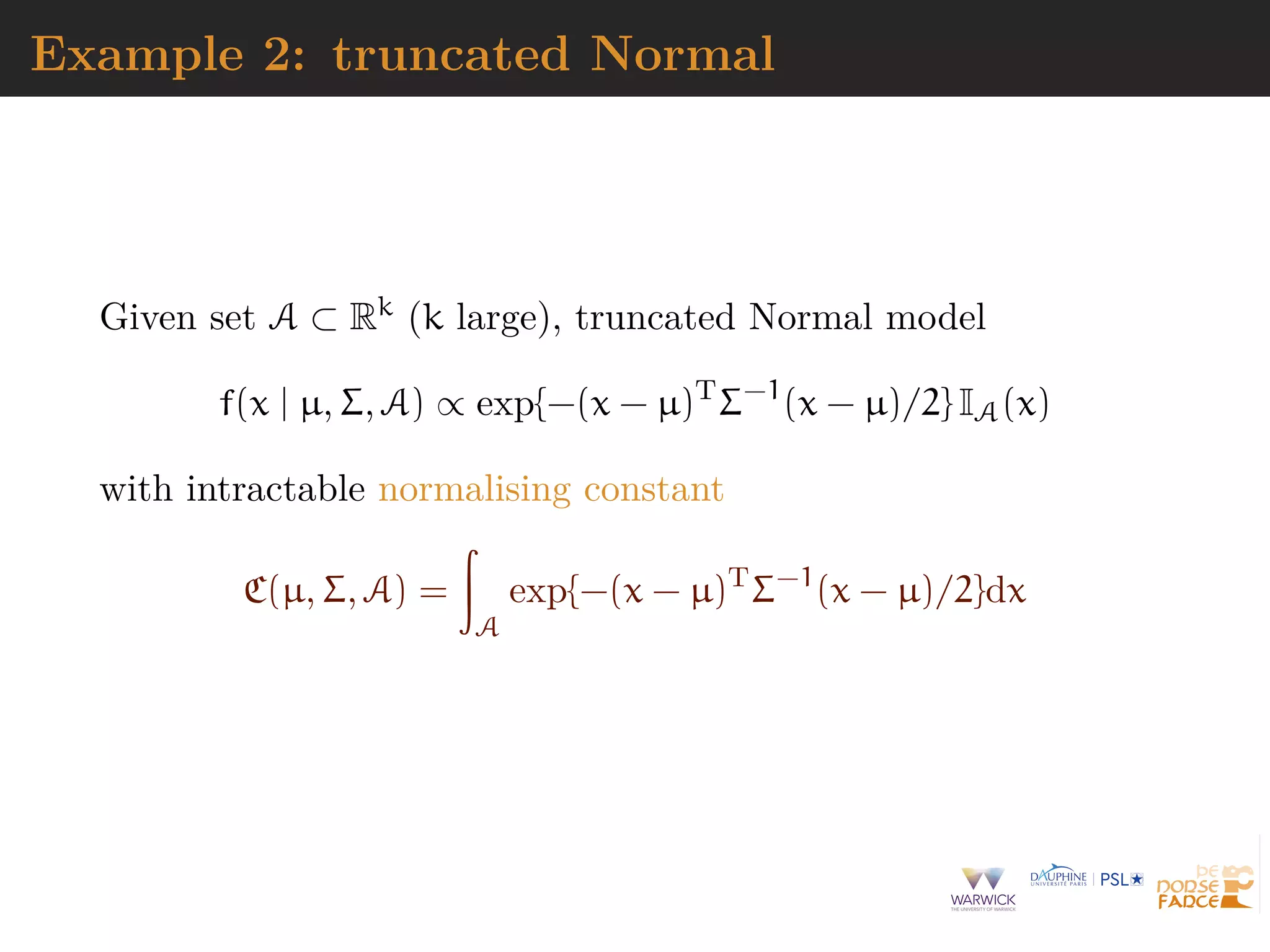
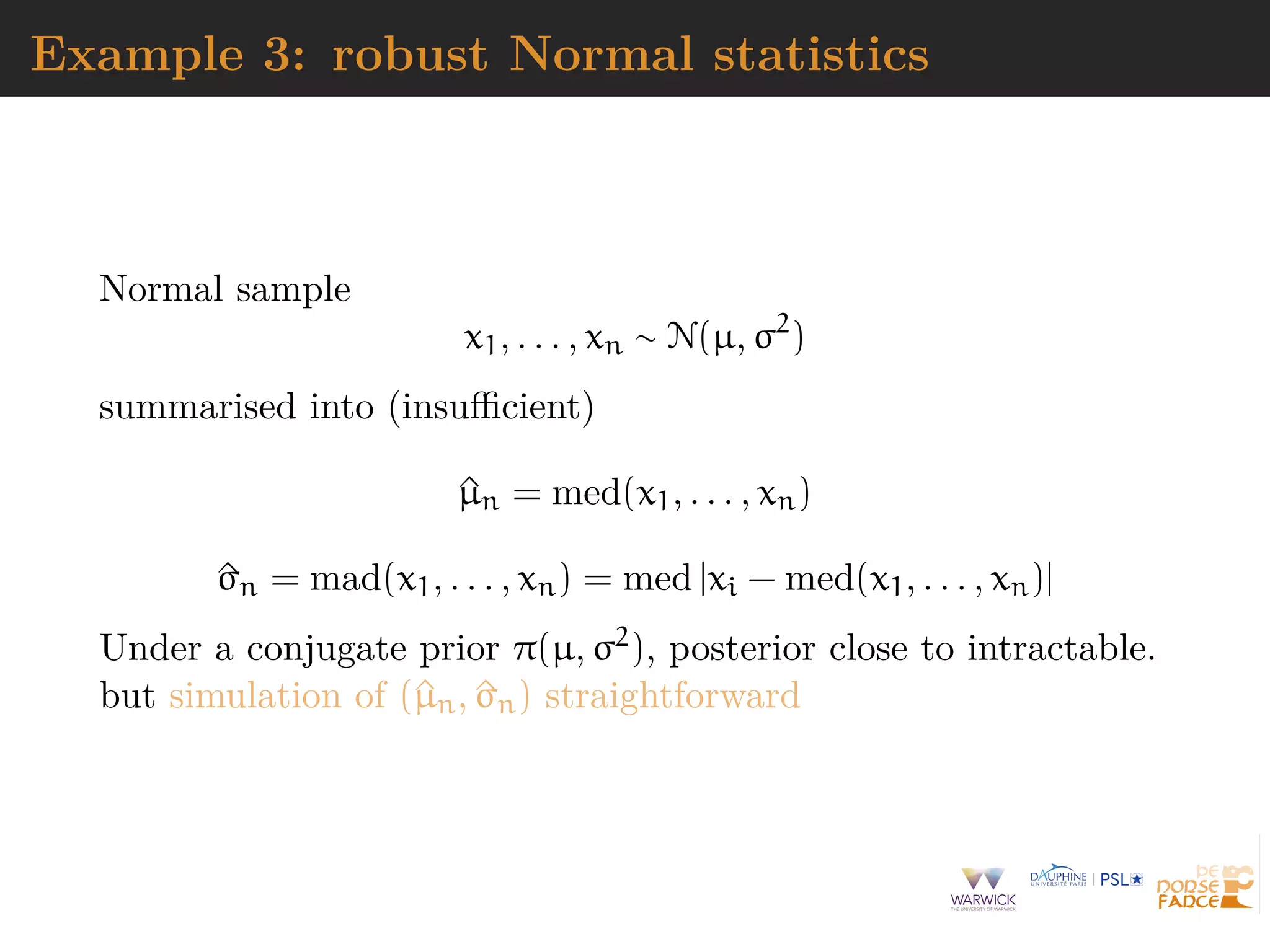
![Example 3: robust Normal statistics
mu=rnorm(N<-1e6) #prior
sig=1/sqrt(rgamma(N,2,2))
medobs=median(obs) #summary
madobs=mad(obs)
for(t in diz<-1:N){
psud=rnorm(1e2)*sig[t]+mu[t]
medpsu=median(psud)-medobs
madpsu=mad(psud)-madobs
diz[t]=medpsuˆ2+madpsuˆ2}
#ABC sample
subz=which(diz<quantile(diz,.1))
plot(mu[subz],sig[subz])](https://image.slidesharecdn.com/jsm19-190720162758/75/the-ABC-of-ABC-20-2048.jpg)
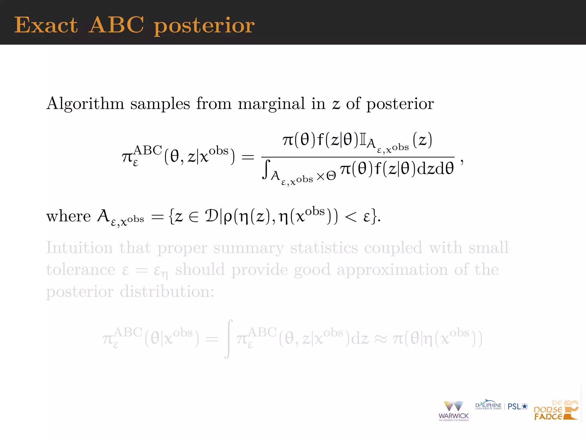
![Why does it work?
The mathematical proof is trivial:
f(θi) ∝
z∈D
π(θi)f(z|θi)Iy(z)
∝ π(θi)f(y|θi)
= π(θi|y) .
[Accept–Reject 101]
But very impractical when
Pθ(Z = xobs
) ≈ 0](https://image.slidesharecdn.com/jsm19-190720162758/75/the-ABC-of-ABC-24-2048.jpg)
![Why does it work?
The mathematical proof is trivial:
f(θi) ∝
z∈D
π(θi)f(z|θi)Iy(z)
∝ π(θi)f(y|θi)
= π(θi|y) .
[Accept–Reject 101]
But very impractical when
Pθ(Z = xobs
) ≈ 0](https://image.slidesharecdn.com/jsm19-190720162758/75/the-ABC-of-ABC-25-2048.jpg)
![A as approximative
When y is a continuous random variable, strict equality
z = xobs is replaced with a tolerance zone
ρ(xobs
, z) ε
where ρ is a distance
Output distributed from
π(θ) Pθ{ρ(xobs
, z) < ε}
def
∝ π(θ|ρ(xobs
, z) < ε)
[Pritchard et al., 1999]](https://image.slidesharecdn.com/jsm19-190720162758/75/the-ABC-of-ABC-26-2048.jpg)
![A as approximative
When y is a continuous random variable, strict equality
z = xobs is replaced with a tolerance zone
ρ(xobs
, z) ε
where ρ is a distance
Output distributed from
π(θ) Pθ{ρ(xobs
, z) < ε}
def
∝ π(θ|ρ(xobs
, z) < ε)
[Pritchard et al., 1999]](https://image.slidesharecdn.com/jsm19-190720162758/75/the-ABC-of-ABC-27-2048.jpg)
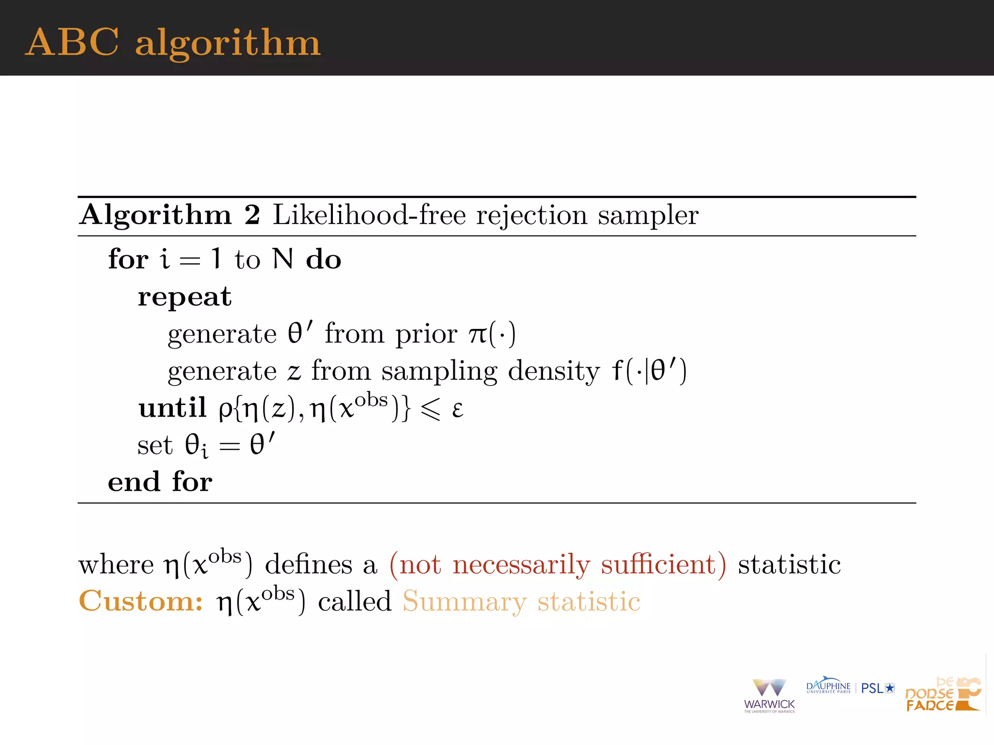
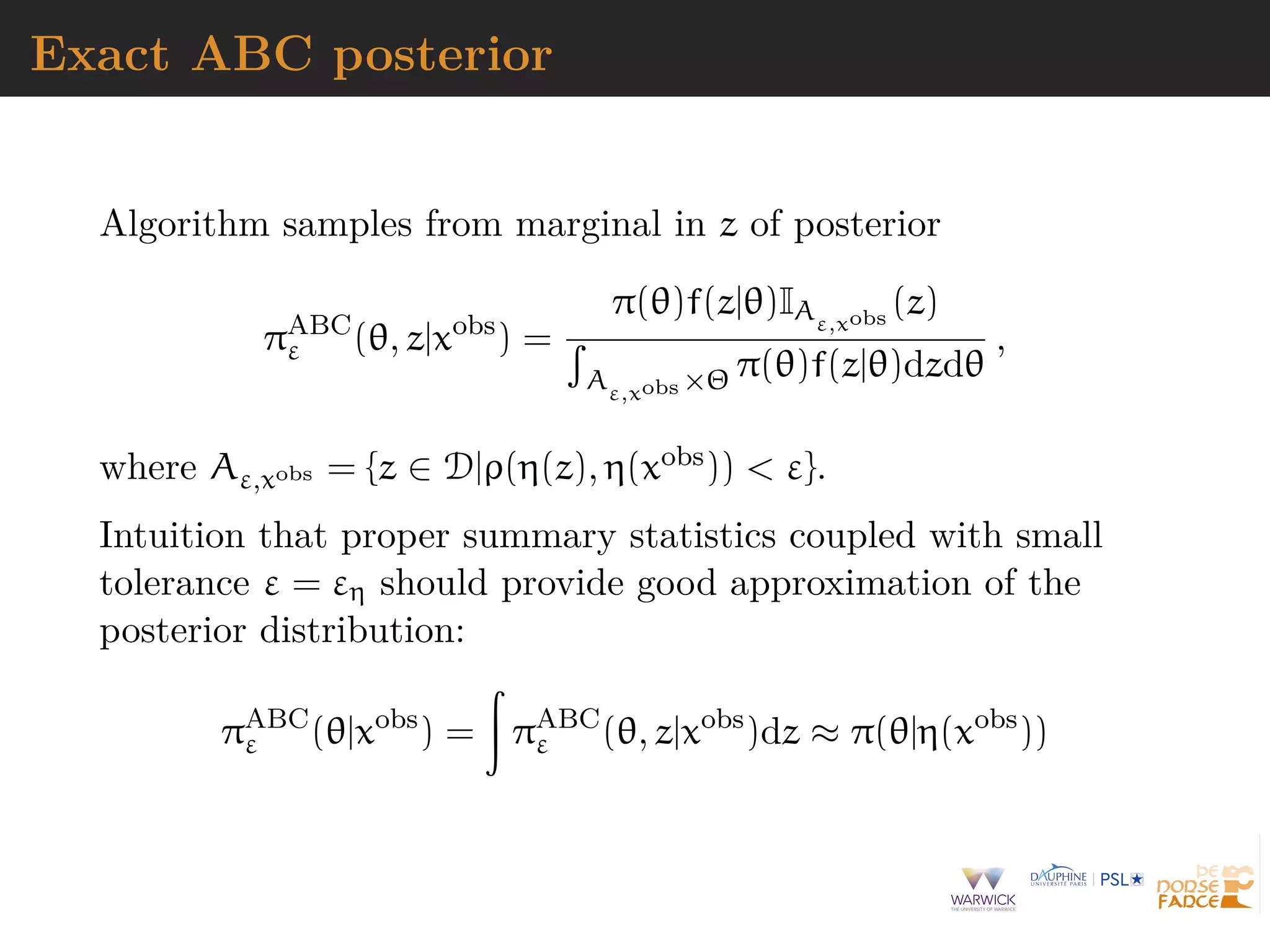
![why not summaries?
loss of sufficient information with πABC(θ|xobs) replaced
with πABC(θ|η(xobs))
arbitrariness of summaries
uncalibrated approximation
whole data may be available (at same cost as summaries)
distributions may be compared (Wasserstein distances)
[Bernton et al., 2019]](https://image.slidesharecdn.com/jsm19-190720162758/75/the-ABC-of-ABC-36-2048.jpg)
![summary strategies
Fundamental difficulty of selecting summary statistics when
there is no non-trivial sufficient statistic [except when done by
experimenters from the field]](https://image.slidesharecdn.com/jsm19-190720162758/75/the-ABC-of-ABC-37-2048.jpg)
![summary strategies
Fundamental difficulty of selecting summary statistics when
there is no non-trivial sufficient statistic [except when done by
experimenters from the field]
1. Starting from large collection of summary statistics, Joyce
and Marjoram (2008) consider the sequential inclusion into the
ABC target, with a stopping rule based on a likelihood ratio
test.](https://image.slidesharecdn.com/jsm19-190720162758/75/the-ABC-of-ABC-38-2048.jpg)
![summary strategies
Fundamental difficulty of selecting summary statistics when
there is no non-trivial sufficient statistic [except when done by
experimenters from the field]
2. Based on decision-theoretic principles, Fearnhead and
Prangle (2012) end up with E[θ|xobs] as the optimal summary
statistic](https://image.slidesharecdn.com/jsm19-190720162758/75/the-ABC-of-ABC-39-2048.jpg)
![summary strategies
Fundamental difficulty of selecting summary statistics when
there is no non-trivial sufficient statistic [except when done by
experimenters from the field]
3. Use of indirect inference by Drovandi, Pettit, & Paddy
(2011) with estimators of parameters of auxiliary model as
summary statistics.](https://image.slidesharecdn.com/jsm19-190720162758/75/the-ABC-of-ABC-40-2048.jpg)
![summary strategies
Fundamental difficulty of selecting summary statistics when
there is no non-trivial sufficient statistic [except when done by
experimenters from the field]
4. Starting from large collection of summary statistics, Raynal
& al. (2018, 2019) rely on random forests to build estimators
and select summaries](https://image.slidesharecdn.com/jsm19-190720162758/75/the-ABC-of-ABC-41-2048.jpg)
![summary strategies
Fundamental difficulty of selecting summary statistics when
there is no non-trivial sufficient statistic [except when done by
experimenters from the field]
5. Starting from large collection of summary statistics, Sedki &
Pudlo (2012) use the Lasso to eliminate summaries](https://image.slidesharecdn.com/jsm19-190720162758/75/the-ABC-of-ABC-42-2048.jpg)
![Semi-automated ABC
Use of summary statistic η(·), importance proposal g(·), kernel
K(·) 1 with bandwidth h ↓ 0 such that
(θ, z) ∼ g(θ)f(z|θ)
accepted with probability (hence the bound)
K[{η(z) − η(xobs
)}/h]
and the corresponding importance weight defined by
π(θ) g(θ)
Theorem Optimality of posterior expectation E[θ|xobs] of
parameter of interest as summary statistics η(xobs)
[Fearnhead & Prangle, 2012; Sisson et al., 2019]](https://image.slidesharecdn.com/jsm19-190720162758/75/the-ABC-of-ABC-43-2048.jpg)
![Semi-automated ABC
Use of summary statistic η(·), importance proposal g(·), kernel
K(·) 1 with bandwidth h ↓ 0 such that
(θ, z) ∼ g(θ)f(z|θ)
accepted with probability (hence the bound)
K[{η(z) − η(xobs
)}/h]
and the corresponding importance weight defined by
π(θ) g(θ)
Theorem Optimality of posterior expectation E[θ|xobs] of
parameter of interest as summary statistics η(xobs)
[Fearnhead & Prangle, 2012; Sisson et al., 2019]](https://image.slidesharecdn.com/jsm19-190720162758/75/the-ABC-of-ABC-44-2048.jpg)
![Random forests
Technique that stemmed from Leo Breiman’s bagging (or
bootstrap aggregating) machine learning algorithm for both
classification [testing] and regression [estimation]
[Breiman, 1996]
Improved performances by averaging over classification schemes
of randomly generated training sets, creating a “forest” of
(CART) decision trees, inspired by Amit and Geman (1997)
ensemble learning
[Breiman, 2001]](https://image.slidesharecdn.com/jsm19-190720162758/75/the-ABC-of-ABC-45-2048.jpg)
![Growing the forest
Breiman’s solution for inducing random features in the trees of
the forest:
boostrap resampling of the dataset and
random subset-ing [of size
√
t] of the covariates driving the
classification or regression at every node of each tree
Covariate (summary) xτ that drives the node separation
xτ cτ
and the separation bound cτ chosen by minimising entropy or
Gini index](https://image.slidesharecdn.com/jsm19-190720162758/75/the-ABC-of-ABC-46-2048.jpg)

![Classification of summaries by random forests
Given large collection of summary statistics, rather than
selecting a subset and excluding the others, estimate each
parameter random forests
handles thousands of predictors
ignores useless components
fast estimation with good local properties
automatised with few calibration steps
substitute to Fearnhead and Prangle (2012) preliminary
estimation of ^θ(yobs)
includes a natural (classification) distance measure that
avoids choice of either distance or tolerance
[Marin et al., 2016]](https://image.slidesharecdn.com/jsm19-190720162758/75/the-ABC-of-ABC-51-2048.jpg)
![Calibration of tolerance
Calibration of threshold ε
from scratch [how small is small?]
from k-nearest neighbour perspective [quantile of prior
predictive]
from asymptotics [convergence speed]
related with choice of distance [automated selection by
random forests]
[Fearnhead & Prangle, 1992; Wilkinson, 2013; Liu & Fearnhead 2018]](https://image.slidesharecdn.com/jsm19-190720162758/75/the-ABC-of-ABC-52-2048.jpg)
![Sofware
Several abc R packages for performing parameter estimation
and model selection
[Nunes & Prangle, 2017]](https://image.slidesharecdn.com/jsm19-190720162758/75/the-ABC-of-ABC-54-2048.jpg)
![Sofware
Several abc R packages for performing parameter estimation
and model selection
[Nunes & Prangle, 2017]
abctools R package tuning ABC analyses](https://image.slidesharecdn.com/jsm19-190720162758/75/the-ABC-of-ABC-55-2048.jpg)
![Sofware
Several abc R packages for performing parameter estimation
and model selection
[Nunes & Prangle, 2017]
abcrf R package ABC via random forests](https://image.slidesharecdn.com/jsm19-190720162758/75/the-ABC-of-ABC-56-2048.jpg)
![Sofware
Several abc R packages for performing parameter estimation
and model selection
[Nunes & Prangle, 2017]
EasyABC R package several algorithms for performing
efficient ABC sampling schemes, including four sequential
sampling schemes and 3 MCMC schemes](https://image.slidesharecdn.com/jsm19-190720162758/75/the-ABC-of-ABC-57-2048.jpg)
![Sofware
Several abc R packages for performing parameter estimation
and model selection
[Nunes & Prangle, 2017]
DIYABC non R software for population genetics](https://image.slidesharecdn.com/jsm19-190720162758/75/the-ABC-of-ABC-58-2048.jpg)
![ABC-IS
Basic ABC algorithm suggests simulating from the prior
blind [no learning]
inefficient [curse of simension]
inapplicable to improper priors
Importance sampling version
importance density g(θ)
bounded kernel function Kh with bandwidth h
acceptance probability of
Kh{ρ[η(xobs
), η(x{θ})]} π(θ) g(θ) max
θ
Aθ
[Fearnhead & Prangle, 2012]](https://image.slidesharecdn.com/jsm19-190720162758/75/the-ABC-of-ABC-59-2048.jpg)
![ABC-IS
Basic ABC algorithm suggests simulating from the prior
blind [no learning]
inefficient [curse of simension]
inapplicable to improper priors
Importance sampling version
importance density g(θ)
bounded kernel function Kh with bandwidth h
acceptance probability of
Kh{ρ[η(xobs
), η(x{θ})]} π(θ) g(θ) max
θ
Aθ
[Fearnhead & Prangle, 2012]](https://image.slidesharecdn.com/jsm19-190720162758/75/the-ABC-of-ABC-60-2048.jpg)
![ABC-MCMC
Markov chain (θ(t)) created via transition function
θ(t+1)
=
θ ∼ Kω(θ |θ(t)) if x ∼ f(x|θ ) is such that x = y
and u ∼ U(0, 1) π(θ )Kω(θ(t)|θ )
π(θ(t))Kω(θ |θ(t))
,
θ(t) otherwise,
has the posterior π(θ|y) as stationary distribution
[Marjoram et al, 2003]](https://image.slidesharecdn.com/jsm19-190720162758/75/the-ABC-of-ABC-61-2048.jpg)
![ABC-MCMC
Algorithm 3 Likelihood-free MCMC sampler
get (θ(0), z(0)) by Algorithm 1
for t = 1 to N do
generate θ from Kω ·|θ(t−1) , z from f(·|θ ), u from U[0,1],
if u π(θ )Kω(θ(t−1)|θ )
π(θ(t−1)Kω(θ |θ(t−1))
IAε,xobs
(z ) then
set (θ(t), z(t)) = (θ , z )
else
(θ(t), z(t))) = (θ(t−1), z(t−1)),
end if
end for](https://image.slidesharecdn.com/jsm19-190720162758/75/the-ABC-of-ABC-62-2048.jpg)
![ABC-PMC
Generate a sample at iteration t by
^πt(θ(t)
) ∝
N
j=1
ω
(t−1)
j Kt(θ(t)
|θ
(t−1)
j )
modulo acceptance of the associated xt, with tolerance εt ↓, and
use importance weight associated with accepted simulation θ
(t)
i
ω
(t)
i ∝ π(θ
(t)
i ) ^πt(θ
(t)
i )
c Still likelihood free
[Sisson et al., 2007; Beaumont et al., 2009]](https://image.slidesharecdn.com/jsm19-190720162758/75/the-ABC-of-ABC-63-2048.jpg)
![ABC-SMC
Use of a kernel Kt associated with target πεt and derivation of
the backward kernel
Lt−1(z, z ) =
πεt (z )Kt(z , z)
πεt (z)
Update of the weights
ω
(t)
i ∝ ω
(t−1)
i
M
m=1 IAεt
(x
(t)
im )
M
m=1 IAεt−1
(x
(t−1)
im )
when x
(t)
im ∼ Kt(x
(t−1)
i , ·)
[Del Moral, Doucet & Jasra, 2009]](https://image.slidesharecdn.com/jsm19-190720162758/75/the-ABC-of-ABC-64-2048.jpg)
![ABC-NP
Better usage of [prior] simulations by
adjustement: instead of throwing
away θ such that ρ(η(z), η(xobs)) > ε,
replace θ’s with locally regressed
transforms
θ∗
= θ − {η(z) − η(xobs
)}T ^β [Csill´ery et al., TEE, 2010]
where ^β is obtained by [NP] weighted least square regression on
(η(z) − η(xobs)) with weights
Kδ ρ(η(z), η(xobs
))
[Beaumont et al., 2002, Genetics]](https://image.slidesharecdn.com/jsm19-190720162758/75/the-ABC-of-ABC-65-2048.jpg)
![ABC-NP (regression)
Also found in the subsequent literature, e.g. in Fearnhead
& Prangle (2012): weight directly simulation by
Kδ ρ[η(z(θ)), η(xobs
)]
or
1
S
S
s=1
Kδ ρ[η(zs
(θ)), η(xobs
)]
[consistent estimate of f(η|θ)]
Curse of dimensionality: poor when d = dim(η) large](https://image.slidesharecdn.com/jsm19-190720162758/75/the-ABC-of-ABC-66-2048.jpg)
![ABC-NP (regression)
Also found in the subsequent literature, e.g. in Fearnhead
& Prangle (2012): weight directly simulation by
Kδ ρ[η(z(θ)), η(xobs
)]
or
1
S
S
s=1
Kδ ρ[η(zs
(θ)), η(xobs
)]
[consistent estimate of f(η|θ)]
Curse of dimensionality: poor when d = dim(η) large](https://image.slidesharecdn.com/jsm19-190720162758/75/the-ABC-of-ABC-67-2048.jpg)
![ABC-NP (density estimation)
Use of the kernel weights
Kδ ρ[η(z(θ)), η(xobs
)]
leads to the NP estimate of the posterior expectation
EABC
[θ | xobs
] ≈ i θiKδ ρ[η(z(θi)), η(xobs)]
i Kδ {ρ[η(z(θi)), η(xobs)]}
[Blum, JASA, 2010]](https://image.slidesharecdn.com/jsm19-190720162758/75/the-ABC-of-ABC-68-2048.jpg)
![ABC-NP (density estimation)
Use of the kernel weights
Kδ ρ[η(z(θ)), η(xobs
)]
leads to the NP estimate of the posterior conditional density
πABC
[θ | xobs
] ≈ i
˜Kb(θi − θ)Kδ ρ[η(z(θi)), η(xobs)]
i Kδ {ρ[η(z(θi)), η(xobs)]}
[Blum, JASA, 2010]](https://image.slidesharecdn.com/jsm19-190720162758/75/the-ABC-of-ABC-69-2048.jpg)
![ABC-NP (density estimations)
Other versions incorporating regression adjustments
i
˜Kb(θ∗
i − θ)Kδ ρ[η(z(θi)), η(xobs)]
i Kδ {ρ[η(z(θi)), η(xobs)]}
In all cases, error
E[^g(θ|xobs
)] − g(θ|xobs
) = cb2
+ cδ2
+ OP(b2
+ δ2
) + OP(1/nδd
)
var(^g(θ|xobs
)) =
c
nbδd
(1 + oP(1))](https://image.slidesharecdn.com/jsm19-190720162758/75/the-ABC-of-ABC-70-2048.jpg)
![ABC-NP (density estimations)
Other versions incorporating regression adjustments
i
˜Kb(θ∗
i − θ)Kδ ρ[η(z(θi)), η(xobs)]
i Kδ {ρ[η(z(θi)), η(xobs)]}
In all cases, error
E[^g(θ|xobs
)] − g(θ|xobs
) = cb2
+ cδ2
+ OP(b2
+ δ2
) + OP(1/nδd
)
var(^g(θ|xobs
)) =
c
nbδd
(1 + oP(1))
[Blum, JASA, 2010]](https://image.slidesharecdn.com/jsm19-190720162758/75/the-ABC-of-ABC-71-2048.jpg)
![ABC-NP (density estimations)
Other versions incorporating regression adjustments
i
˜Kb(θ∗
i − θ)Kδ ρ[η(z(θi)), η(xobs)]
i Kδ {ρ[η(z(θi)), η(xobs)]}
In all cases, error
E[^g(θ|xobs
)] − g(θ|xobs
) = cb2
+ cδ2
+ OP(b2
+ δ2
) + OP(1/nδd
)
var(^g(θ|xobs
)) =
c
nbδd
(1 + oP(1))
[standard NP calculations]](https://image.slidesharecdn.com/jsm19-190720162758/75/the-ABC-of-ABC-72-2048.jpg)
![ABC-NCH
Incorporating non-linearities and heterocedasticities:
θ∗
= ^m(η(xobs
)) + [θ − ^m(η(z))]
^σ(η(xobs))
^σ(η(z))
where
^m(η) estimated by non-linear regression (e.g., neural
network)
^σ(η) estimated by non-linear regression on residuals
log{θi − ^m(ηi)}2
= log σ2
(ηi) + ξi
[Blum & Franc¸ois, 2009]](https://image.slidesharecdn.com/jsm19-190720162758/75/the-ABC-of-ABC-73-2048.jpg)
![ABC-NCH
Incorporating non-linearities and heterocedasticities:
θ∗
= ^m(η(xobs
)) + [θ − ^m(η(z))]
^σ(η(xobs))
^σ(η(z))
where
^m(η) estimated by non-linear regression (e.g., neural
network)
^σ(η) estimated by non-linear regression on residuals
log{θi − ^m(ηi)}2
= log σ2
(ηi) + ξi
[Blum & Franc¸ois, 2009]](https://image.slidesharecdn.com/jsm19-190720162758/75/the-ABC-of-ABC-74-2048.jpg)
![ABC-NCH
Why neural network?
fights curse of dimensionality
selects relevant summary statistics
provides automated dimension reduction
offers a model choice capability
improves upon multinomial logistic
[Blum & Franc¸ois, 2009]](https://image.slidesharecdn.com/jsm19-190720162758/75/the-ABC-of-ABC-75-2048.jpg)

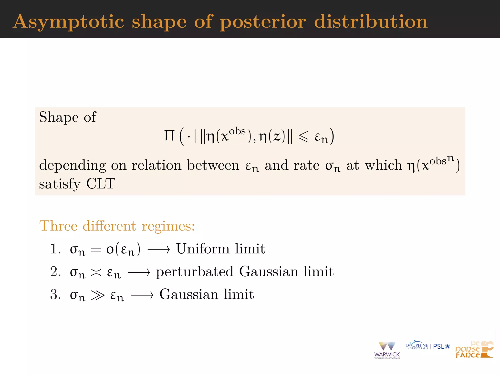
![Asymptotics of ABC
Since πABC(· | xobs) is an approximation of π(· | xobs) or
π(· | η(xobs)) coherence of ABC-based inference need be
established on its own
[Li & Fearnhead, 2018a, 2018b; Frazier et al., 2018]
Meaning
establishing large sample (n) properties of ABC posteriors
and ABC procedures
finding sufficient conditions and checks on summary
statistics η(cdot)
determining proper rate of convergence of tolerance to 0 as
ε = εn
[mostly] ignoring Monte Carlo errors](https://image.slidesharecdn.com/jsm19-190720162758/75/the-ABC-of-ABC-77-2048.jpg)
![Asymptotics of ABC
Since πABC(· | xobs) is an approximation of π(· | xobs) or
π(· | η(xobs)) coherence of ABC-based inference need be
established on its own
[Li & Fearnhead, 2018a, 2018b; Frazier et al., 2018]
Meaning
establishing large sample (n) properties of ABC posteriors
and ABC procedures
finding sufficient conditions and checks on summary
statistics η(cdot)
determining proper rate of convergence of tolerance to 0 as
ε = εn
[mostly] ignoring Monte Carlo errors](https://image.slidesharecdn.com/jsm19-190720162758/75/the-ABC-of-ABC-78-2048.jpg)
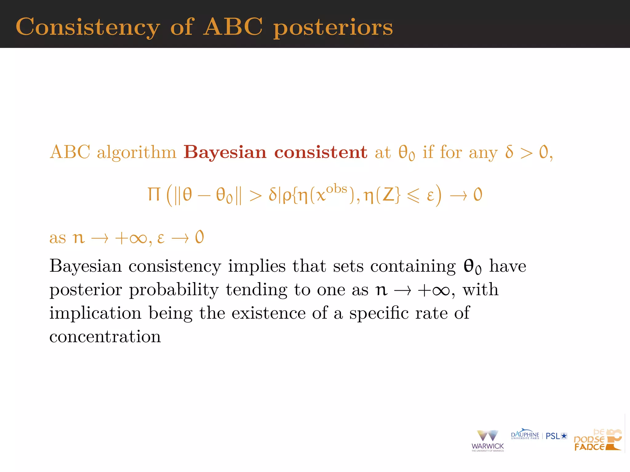
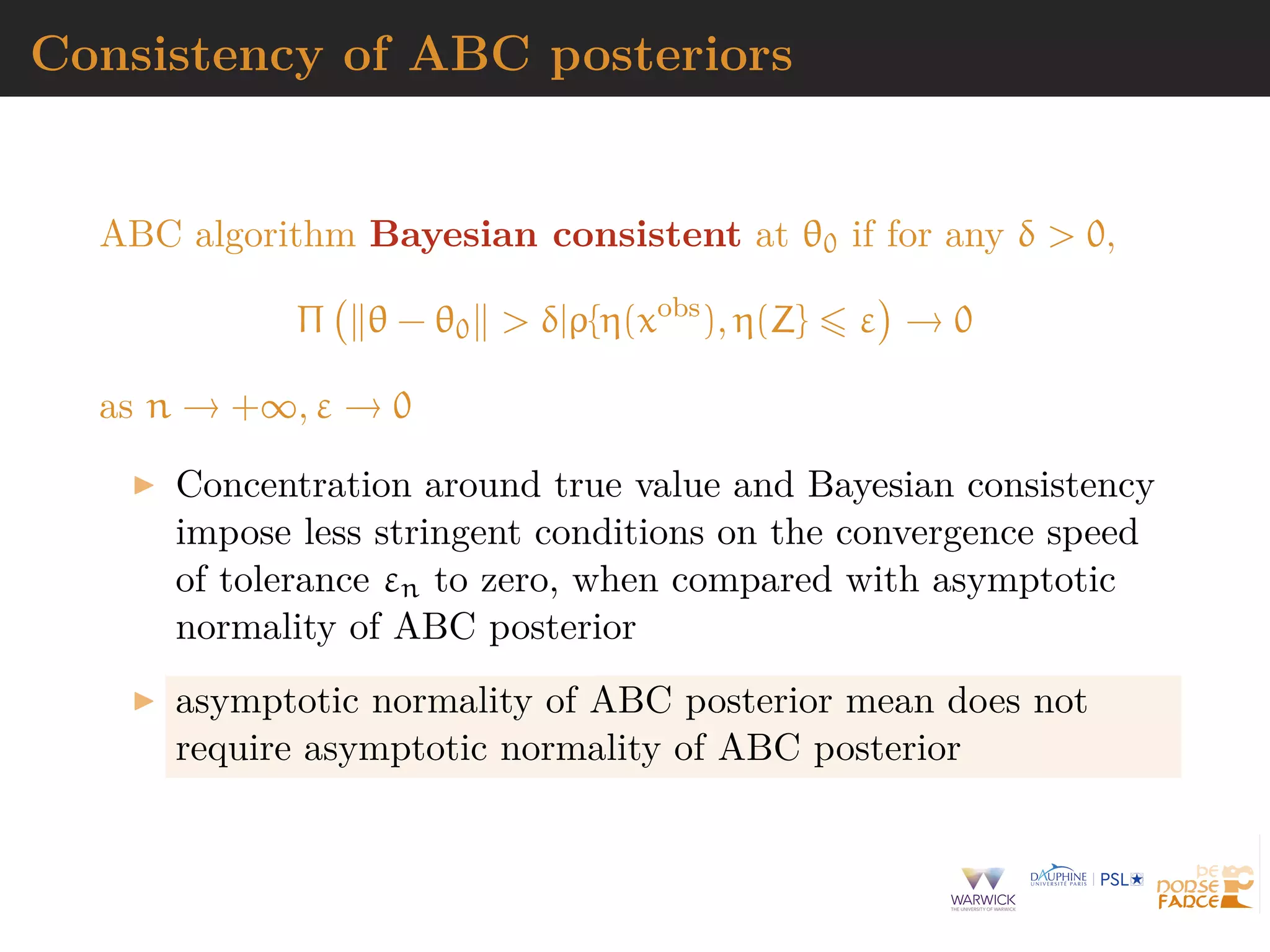

![Consistency of ABC posteriors
Consistency:
Πεn θ − θ0 δ|η(xobs
) = 1 + op(1)
Convergence rate: there exists δn = o(1) such that
Πεn θ − θ0 δn|η(xobs
) = 1 + op(1)
Point estimator consistency
^θε = EABC[θ|η(xobs(n)
)], EABC[θ|η(xobs(n)
)] − θ0 = op(1)
vn(EABC[θ|η(xobs(n)
)] − θ0) ⇒ N(0, v)](https://image.slidesharecdn.com/jsm19-190720162758/75/the-ABC-of-ABC-83-2048.jpg)
![Related convergence results
Studies on the large sample properties of ABC, with focus the
asymptotic properties of ABC point estimators
[Creel et al., 2015; Jasra, 2015; Li & Fearnhead, 2018a,b]
assumption of CLT for summary statistic plus regularity
assumptions on convergence of its density to Normal limit
convergence rate of posterior mean if εT = o(1/v
3/5
T )
acceptance probability chosen as arbitrary density
η(xobs) − η(z)](https://image.slidesharecdn.com/jsm19-190720162758/75/the-ABC-of-ABC-84-2048.jpg)
![Related convergence results
Studies on the large sample properties of ABC, with focus the
asymptotic properties of ABC point estimators
[Creel et al., 2015; Jasra, 2015; Li & Fearnhead, 2018a,b]
characterisation of asymptotic behavior of ABC posterior
for all εT = o(1) with posterior concentration
asymptotic normality and unbiasedness of posterior mean
remain achievable even when limT vT εT = ∞, provided
εT = o(1/v
1/2
T )](https://image.slidesharecdn.com/jsm19-190720162758/75/the-ABC-of-ABC-85-2048.jpg)
![Related convergence results
Studies on the large sample properties of ABC, with focus the
asymptotic properties of ABC point estimators
[Creel et al., 2015; Jasra, 2015; Li & Fearnhead, 2018a,b]
if kη > kθ 1 and if εT = o(1/v
3/5
T ), posterior mean
asymptotically normal, unbiased, but asymptotically
inefficient
if vT εT → ∞ and vT ε2
T = o(1), for kη > kθ 1,
EΠε {vT (θ−θ0)} = { θb(θ0) θb(θ0)}−1
θb(θ0) vT {η(xobs
)−b(θ0)}+op(1).](https://image.slidesharecdn.com/jsm19-190720162758/75/the-ABC-of-ABC-86-2048.jpg)
![asymptotic behaviour of posterior mean
When p = dim(η(xobs)) = d = dim(θ) and εn = o(n−3/10)
EABC[dT (θ − θ0)|xobs
] ⇒ N(0, ( bo
)T
Σ−1
bo −1
[Li & Fearnhead (2018a)]
In fact, if εβ+1
n
√
n = o(1), with β H¨older-smoothness of π
EABC[(θ−θ0)|xobs
] =
( bo)−1Zo
√
n
+
k
j=1
hj(θ0)ε2j
n +op(1), 2k = β
[Fearnhead & Prangle, 2012]](https://image.slidesharecdn.com/jsm19-190720162758/75/the-ABC-of-ABC-88-2048.jpg)
![asymptotic behaviour of posterior mean
When p = dim(η(xobs)) = d = dim(θ) and εn = o(n−3/10)
EABC[dT (θ − θ0)|xobs
] ⇒ N(0, ( bo
)T
Σ−1
bo −1
[Li & Fearnhead (2018a)]
Iterating for fixed p mildly interesting: if
˜η(xobs) = EABC[θ|xobs
]
then
EABC[θ|˜η(xobs
)] = θ0 +
( bo)−1Zo
√
n
+
π (θ0)
π(θ0)
ε2
n + o()
[Fearnhead & Prangle, 2012]](https://image.slidesharecdn.com/jsm19-190720162758/75/the-ABC-of-ABC-89-2048.jpg)
![Curse of dimensionality
For reasonable statistical behavior, decline of acceptance
αT the faster the larger the dimension of θ, kθ, but
unaffected by dimension of η, kη
Theoretical justification for dimension reduction methods
that process parameter components individually and
independently of other components
[Fearnhead & Prangle, 2012; Martin & al., 2016]
importance sampling approach of Li & Fearnhead (2018a)
yields acceptance rates αT = O(1), when εT = O(1/vT )](https://image.slidesharecdn.com/jsm19-190720162758/75/the-ABC-of-ABC-90-2048.jpg)
![Curse of dimensionality
For reasonable statistical behavior, decline of acceptance
αT the faster the larger the dimension of θ, kθ, but
unaffected by dimension of η, kη
Theoretical justification for dimension reduction methods
that process parameter components individually and
independently of other components
[Fearnhead & Prangle, 2012; Martin & al., 2016]
importance sampling approach of Li & Fearnhead (2018a)
yields acceptance rates αT = O(1), when εT = O(1/vT )](https://image.slidesharecdn.com/jsm19-190720162758/75/the-ABC-of-ABC-91-2048.jpg)
![Monte Carlo error
Link the choice of εT to Monte Carlo error associated with NT
draws in ABC Algorithm
Conditions (on εT ) under which
^αT = αT {1 + op(1)}
where ^αT = NT
i=1 1l [d{η(y), η(z)} εT ] /NT proportion of
accepted draws from NT simulated draws of θ
Either
(i) εT = o(v−1
T ) and (vT εT )−kη ε−kθ
T MNT
or
(ii) εT v−1
T and ε−kθ
T MNT
for M large enough](https://image.slidesharecdn.com/jsm19-190720162758/75/the-ABC-of-ABC-92-2048.jpg)
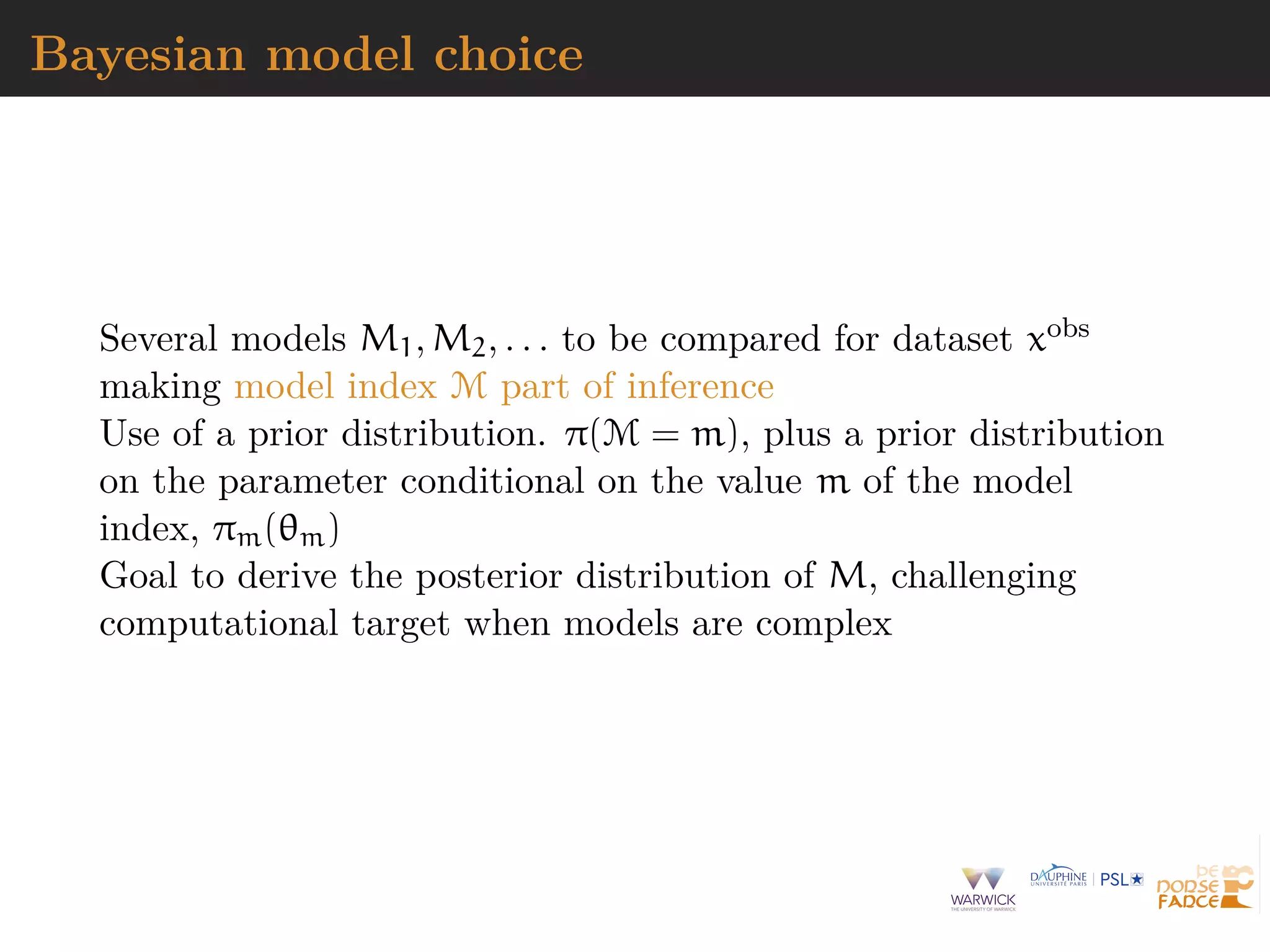
![Generic ABC for model choice
Algorithm 4 Likelihood-free model choice sampler (ABC-MC)
for t = 1 to T do
repeat
Generate m from the prior π(M = m)
Generate θm from the prior πm(θm)
Generate z from the model fm(z|θm)
until ρ{η(z), η(xobs)} < ε
Set m(t) = m and θ(t) = θm
end for
[Cornuet et al., DIYABC, 2009]](https://image.slidesharecdn.com/jsm19-190720162758/75/the-ABC-of-ABC-94-2048.jpg)
![ABC model choice consistency
Leaving approximations aside, limiting ABC procedure is Bayes
factor based on η(xobs)
B12(η(xobs
))
Potential loss of information at the testing level
[Robert et al., 2010]
When is Bayes factor based on insufficient statistic η(xobs)
consistent?
[Marin et al., 2013]](https://image.slidesharecdn.com/jsm19-190720162758/75/the-ABC-of-ABC-95-2048.jpg)
![ABC model choice consistency
Leaving approximations aside, limiting ABC procedure is Bayes
factor based on η(xobs)
B12(η(xobs
))
Potential loss of information at the testing level
[Robert et al., 2010]
When is Bayes factor based on insufficient statistic η(xobs)
consistent?
[Marin et al., 2013]](https://image.slidesharecdn.com/jsm19-190720162758/75/the-ABC-of-ABC-96-2048.jpg)
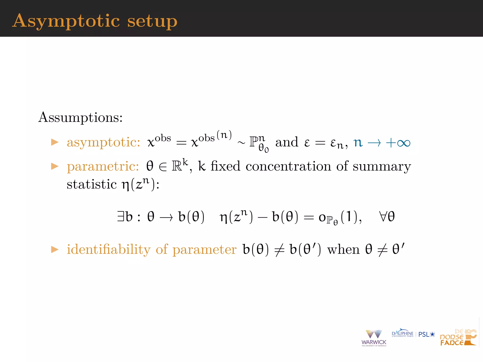
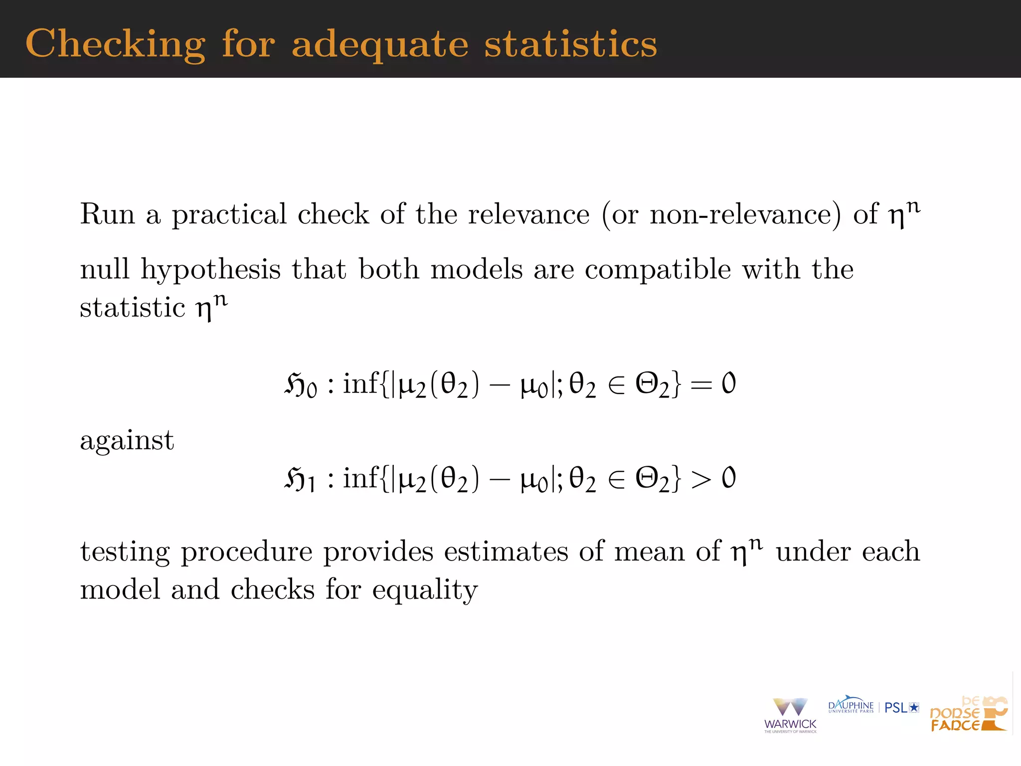
![Consistency
Summary statistics
η(xobs
) = (τ1(xobs
), τ2(xobs
), · · · , τd(xobs
)) ∈ Rd
with true distribution η ∼ Gn, true mean µ0, and distribution
Gi,n under model Mi, corresponding posteriors pi2(· | ηn)
Assumptions of central limit theorem and large deviations for
eta(xobs) under true, plus usual Bayesian asymptotics with di
effective dimension of the parameter)
[Pillai et al., 2013]](https://image.slidesharecdn.com/jsm19-190720162758/75/the-ABC-of-ABC-99-2048.jpg)
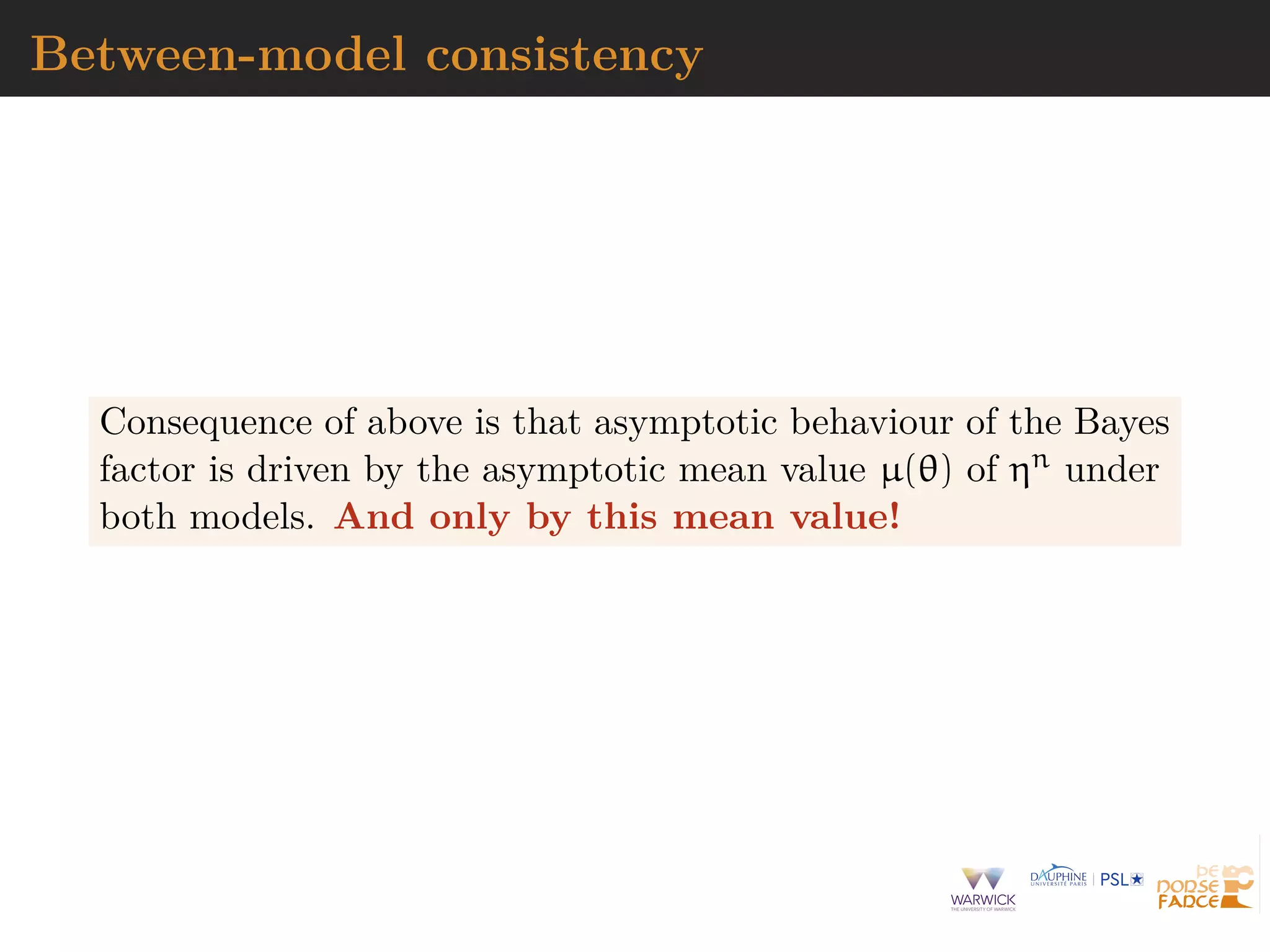
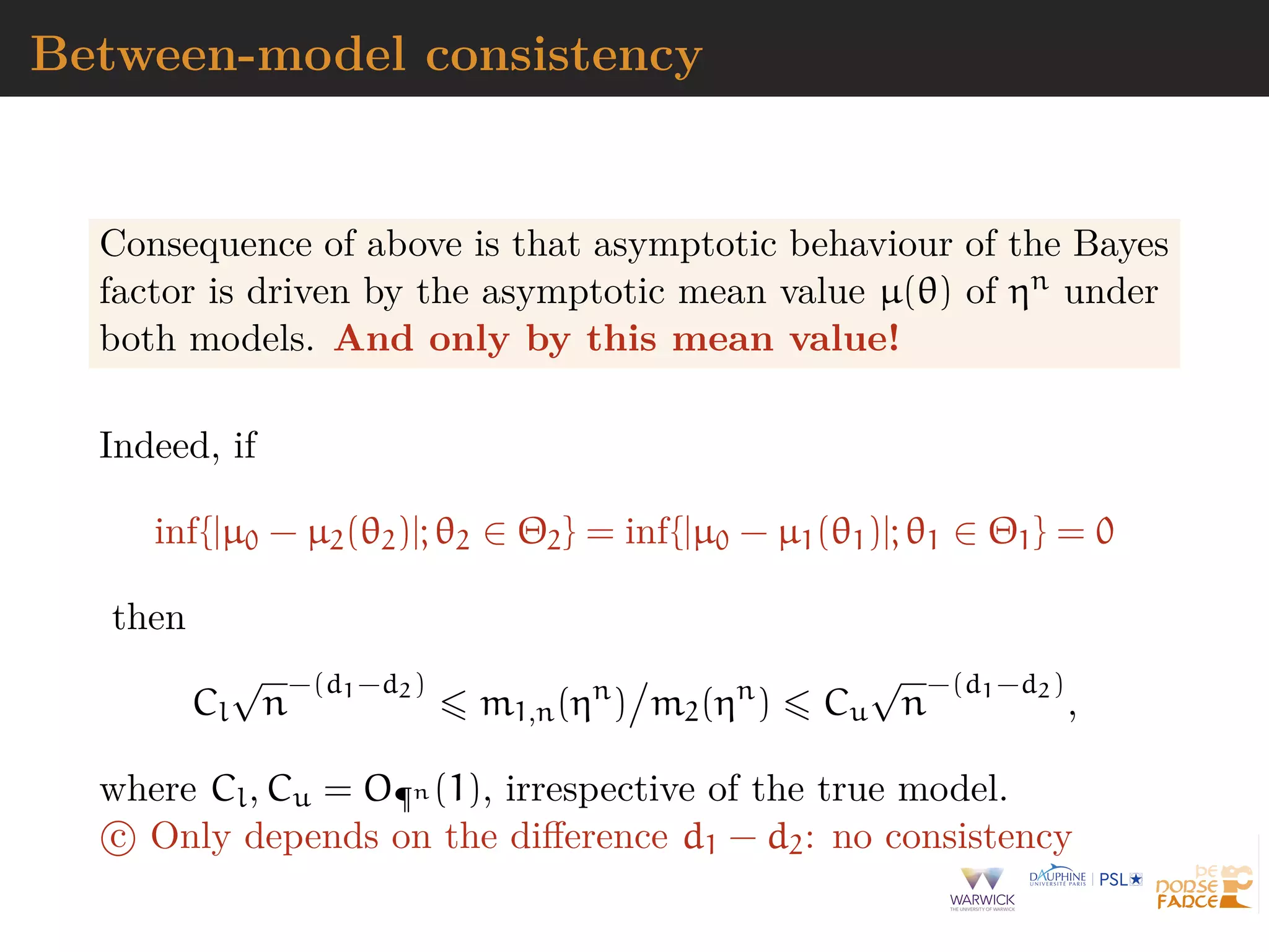
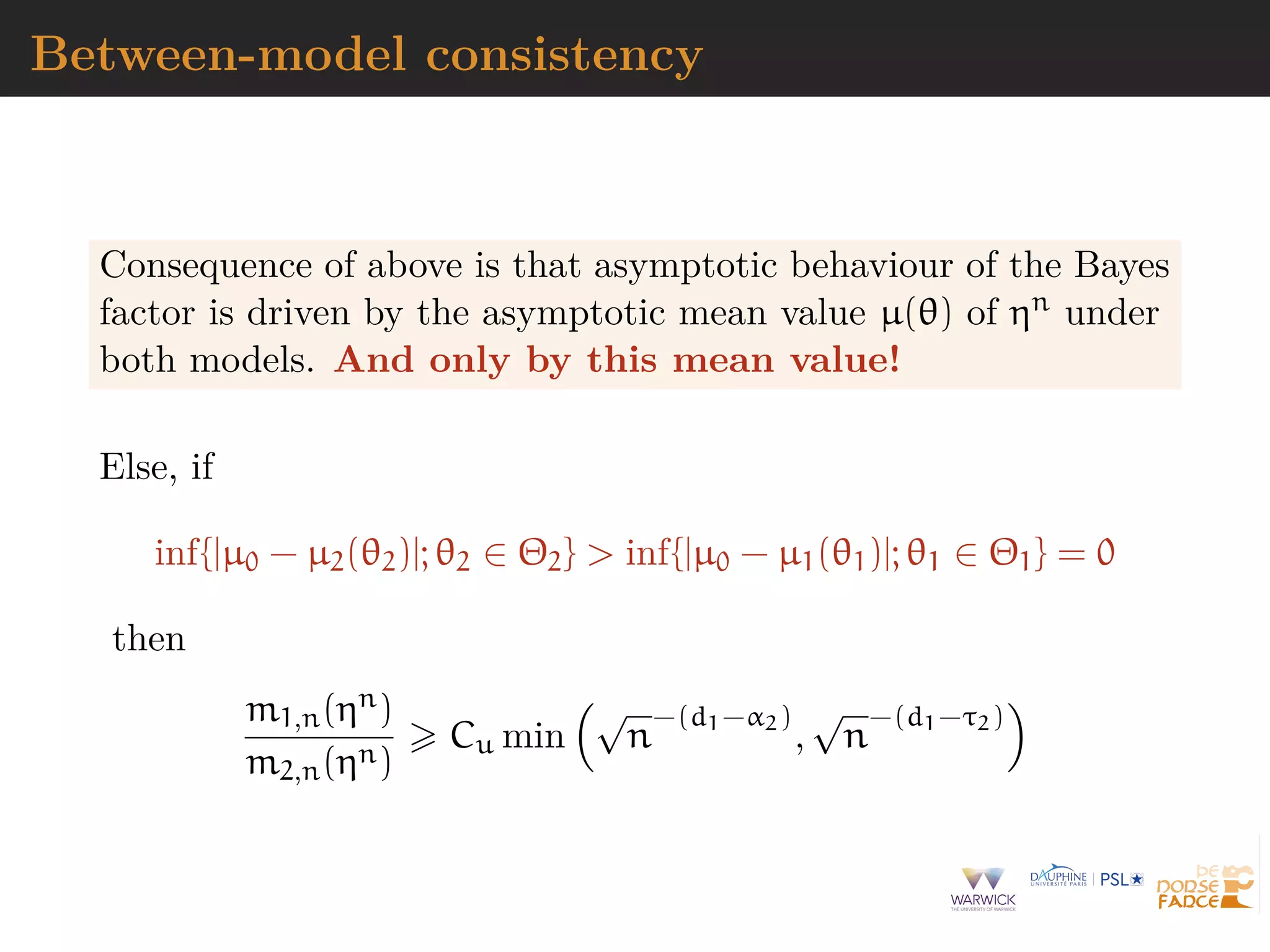
![Asymptotic marginals
Asymptotically
mi,n(t) =
Θi
gi,n(t|θi) πi(θi) dθi
such that
(i) if inf{|µi(θi) − µ0|; θi ∈ Θi} = 0,
Cl
√
n
d−di
mi,n(ηn
) Cu
√
n
d−di
and
(ii) if inf{|µi(θi) − µ0|; θi ∈ Θi} > 0
mi,n(ηn
) = o¶n [
√
n
d−τi
+
√
n
d−αi
].](https://image.slidesharecdn.com/jsm19-190720162758/75/the-ABC-of-ABC-100-2048.jpg)
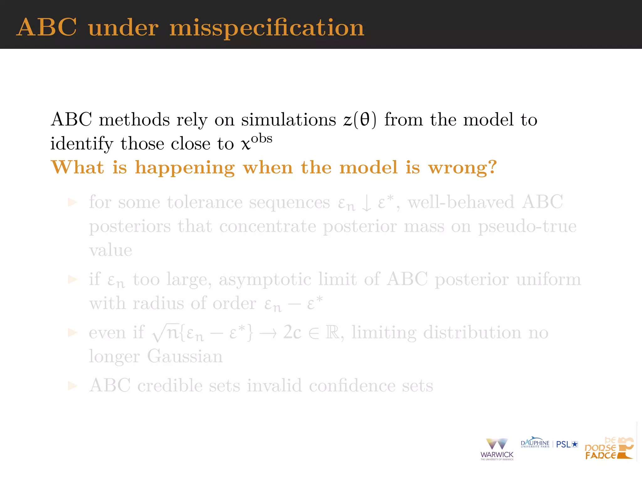
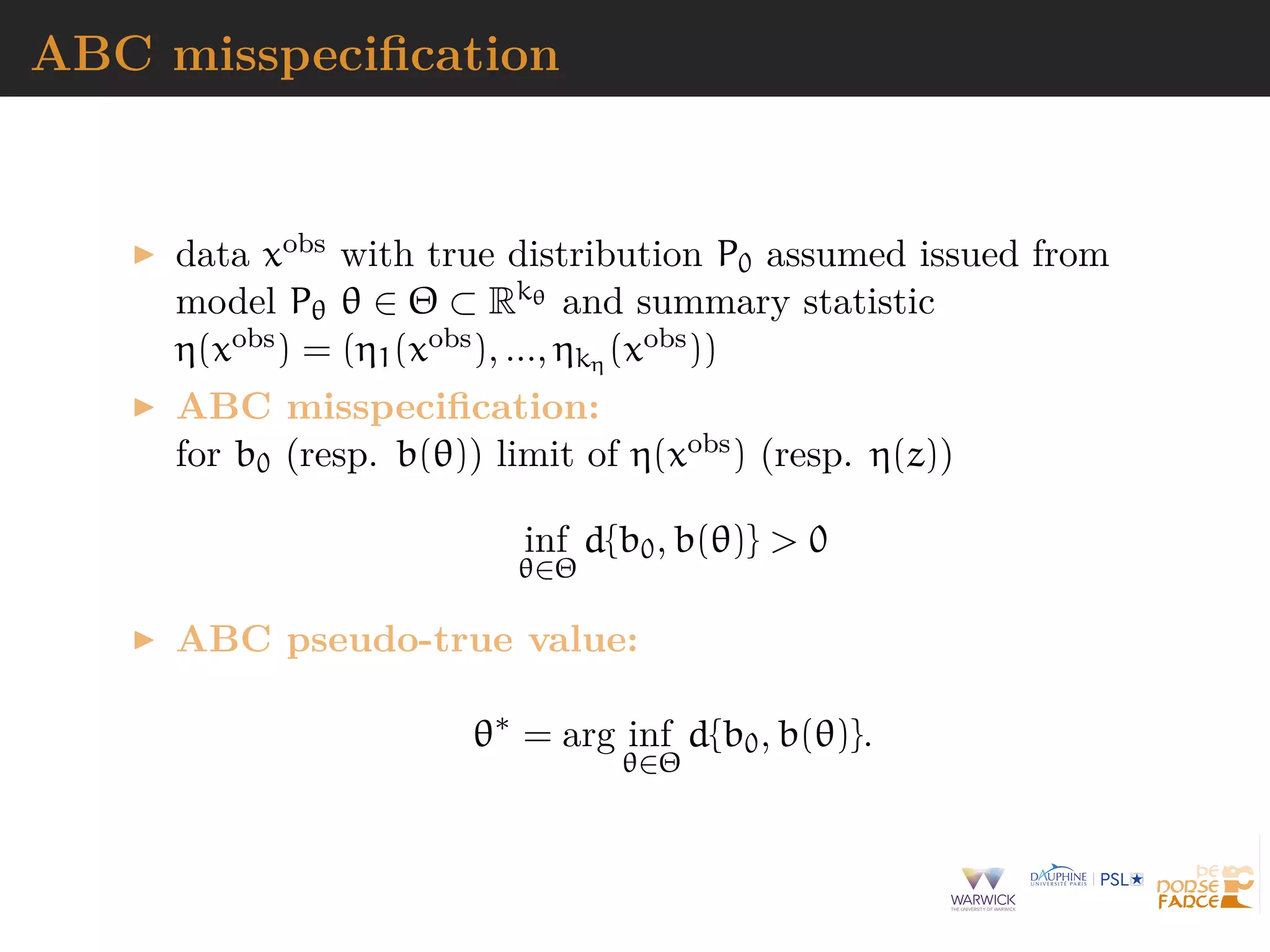
![ABC misspecification
data xobs with true distribution P0 assumed issued from
model Pθ θ ∈ Θ ⊂ Rkθ and summary statistic
η(xobs) = (η1(xobs), ..., ηkη (xobs))
misspecification
inf
θ∈Θ
D(P0||Pθ) = inf
θ∈Θ
log
dP0(x)
dPθ(x)
dP0(y) > 0,
with
θ∗
= arg inf
θ∈Θ
D(P0||Pθ)
[Muller, 2013]
ABC misspecification:
for b0 (resp. b(θ)) limit of η(xobs) (resp. η(z))
inf
θ∈Θ
d{b0, b(θ)} > 0](https://image.slidesharecdn.com/jsm19-190720162758/75/the-ABC-of-ABC-109-2048.jpg)
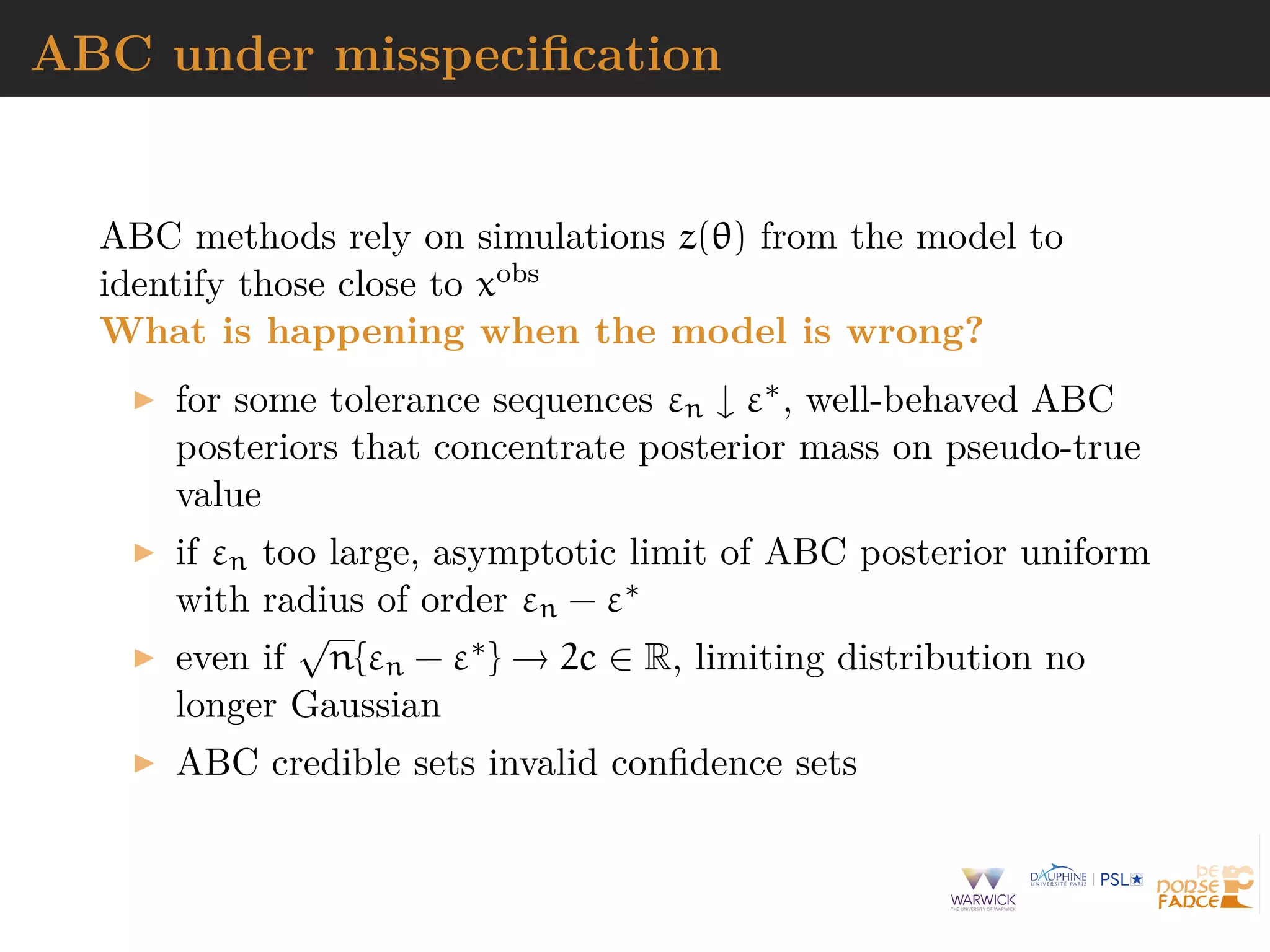
![Minimum tolerance
Approximate nature of ABC means that D(P0||Pθ) yields no
meaningful notion of model misspecification associated with the
output of ABC posterior distributions
Under identification conditions on b(·) ∈ Rkη , there exists ε∗
such that
ε∗
= inf
θ∈Θ
d{b0, b(θ)} > 0
Once εn < ε∗ no draw of θ to be selected and posterior
Πε[A|η(xobs)] ill-conditioned
But appropriately chosen tolerance sequence (εn)n allows
ABC-based posterior to concentrate on distance-dependent
pseudo-true value θ∗](https://image.slidesharecdn.com/jsm19-190720162758/75/the-ABC-of-ABC-111-2048.jpg)
![Minimum tolerance
Approximate nature of ABC means that D(P0||Pθ) yields no
meaningful notion of model misspecification associated with the
output of ABC posterior distributions
Under identification conditions on b(·) ∈ Rkη , there exists ε∗
such that
ε∗
= inf
θ∈Θ
d{b0, b(θ)} > 0
Once εn < ε∗ no draw of θ to be selected and posterior
Πε[A|η(xobs)] ill-conditioned
But appropriately chosen tolerance sequence (εn)n allows
ABC-based posterior to concentrate on distance-dependent
pseudo-true value θ∗](https://image.slidesharecdn.com/jsm19-190720162758/75/the-ABC-of-ABC-112-2048.jpg)
![Minimum tolerance
Approximate nature of ABC means that D(P0||Pθ) yields no
meaningful notion of model misspecification associated with the
output of ABC posterior distributions
Under identification conditions on b(·) ∈ Rkη , there exists ε∗
such that
ε∗
= inf
θ∈Θ
d{b0, b(θ)} > 0
Once εn < ε∗ no draw of θ to be selected and posterior
Πε[A|η(xobs)] ill-conditioned
But appropriately chosen tolerance sequence (εn)n allows
ABC-based posterior to concentrate on distance-dependent
pseudo-true value θ∗](https://image.slidesharecdn.com/jsm19-190720162758/75/the-ABC-of-ABC-113-2048.jpg)
![Minimum tolerance
Approximate nature of ABC means that D(P0||Pθ) yields no
meaningful notion of model misspecification associated with the
output of ABC posterior distributions
Under identification conditions on b(·) ∈ Rkη , there exists ε∗
such that
ε∗
= inf
θ∈Θ
d{b0, b(θ)} > 0
Once εn < ε∗ no draw of θ to be selected and posterior
Πε[A|η(xobs)] ill-conditioned
But appropriately chosen tolerance sequence (εn)n allows
ABC-based posterior to concentrate on distance-dependent
pseudo-true value θ∗](https://image.slidesharecdn.com/jsm19-190720162758/75/the-ABC-of-ABC-114-2048.jpg)
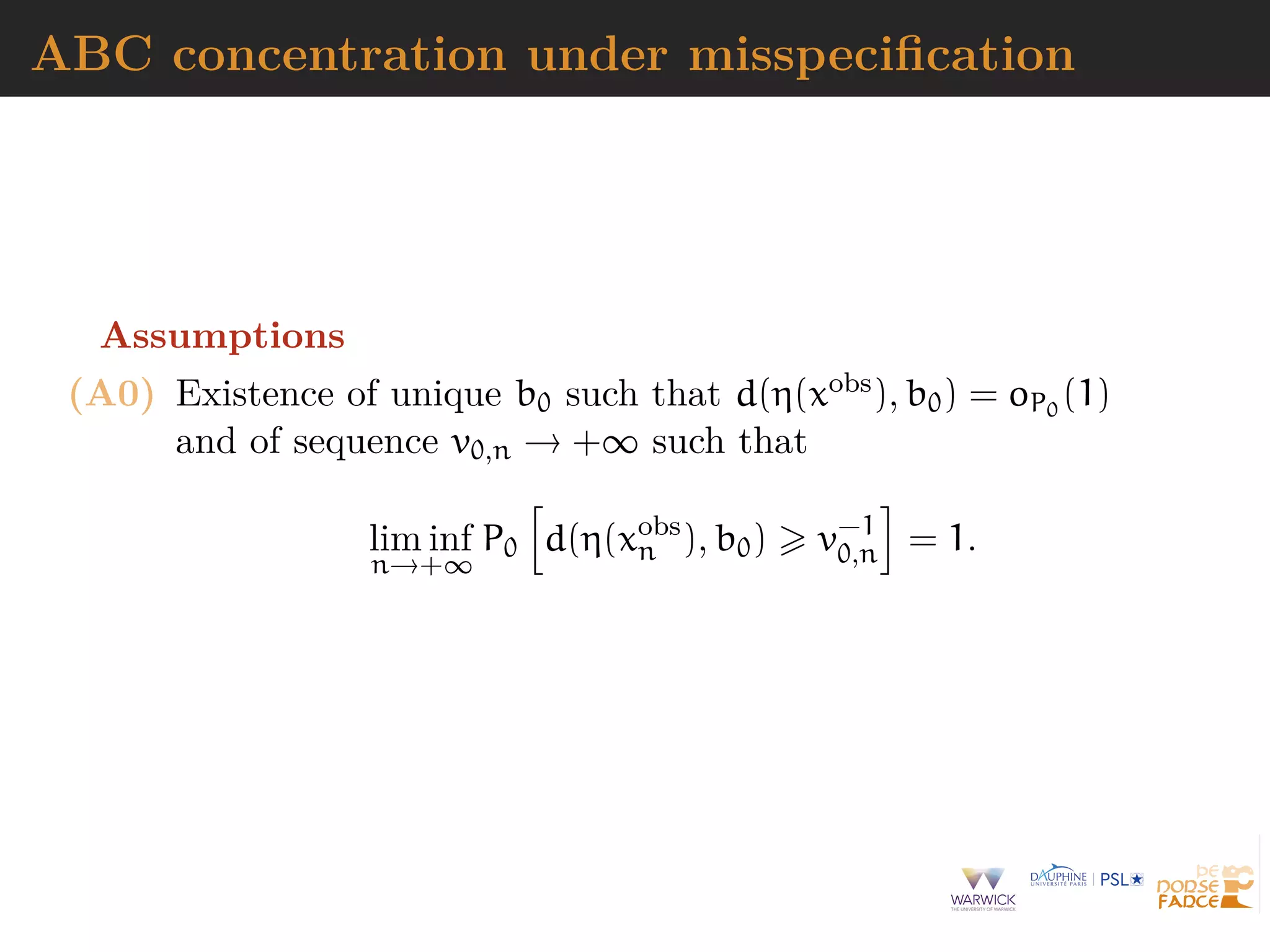
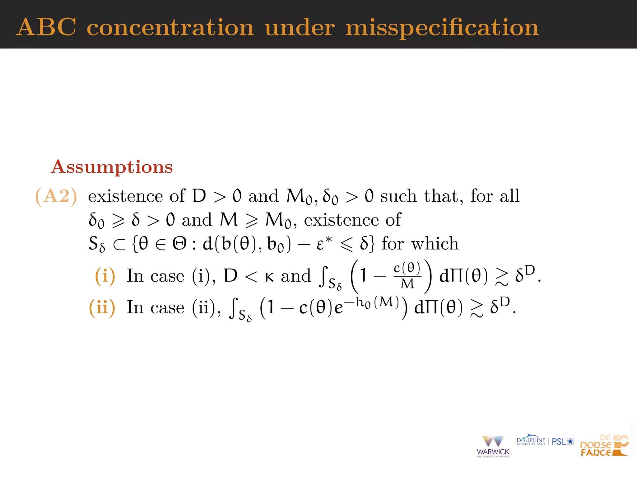
![ABC concentration under misspecification
Assumptions
(A1) Existence of injective map b : Θ → B ⊂ Rkη and function
ρn with ρn(·) ↓ 0 as n → +∞, and ρn(·) non-increasing,
such that
Pθ [d(η(Z), b(θ)) > u] c(θ)ρn(u),
Θ
c(θ)dΠ(θ) < ∞
and assume either
(i) Polynomial deviations: existence of vn ↑ +∞ and
u0, κ > 0 such that ρn(u) = v−κ
n u−κ, for u u0
(ii) Exponential deviations:](https://image.slidesharecdn.com/jsm19-190720162758/75/the-ABC-of-ABC-116-2048.jpg)
![ABC concentration under misspecification
Assumptions
(A1) Existence of injective map b : Θ → B ⊂ Rkη and function
ρn with ρn(·) ↓ 0 as n → +∞, and ρn(·) non-increasing,
such that
Pθ [d(η(Z), b(θ)) > u] c(θ)ρn(u),
Θ
c(θ)dΠ(θ) < ∞
and assume either
(i) Polynomial deviations:
(ii) Exponential deviations: existence of hθ(·) > 0 such
that Pθ[d(η(z), b(θ)) > u] c(θ)e−hθ(uvn) and
existence of m, C > 0 such that
Θ
c(θ)e−hθ(uvn)
dΠ(θ) Ce−m·(uvn)τ
, for u u0.](https://image.slidesharecdn.com/jsm19-190720162758/75/the-ABC-of-ABC-117-2048.jpg)
![Consistency
Assume (A0), [A1] and [A2], with εn ↓ ε∗ with
εn ε∗
+ Mv−1
n + v−1
0,n,
for M large enough. Let Mn ↑ ∞ and δn Mn(εn − ε∗), then
Πε d(b(θ), b0) ε∗
+ δn|η(xobs
) = oP0
(1),
1. if δn Mnv−1
n u
−D/κ
n = o(1) in case (i)
2. if δn Mnv−1
n | log(un)|1/τ = o(1) in case (ii)
with un = εn − (ε∗ + Mv−1
n + v−1
0,n) 0 .
[Bernton et al., 2017; Frazier et al., 2019]](https://image.slidesharecdn.com/jsm19-190720162758/75/the-ABC-of-ABC-119-2048.jpg)
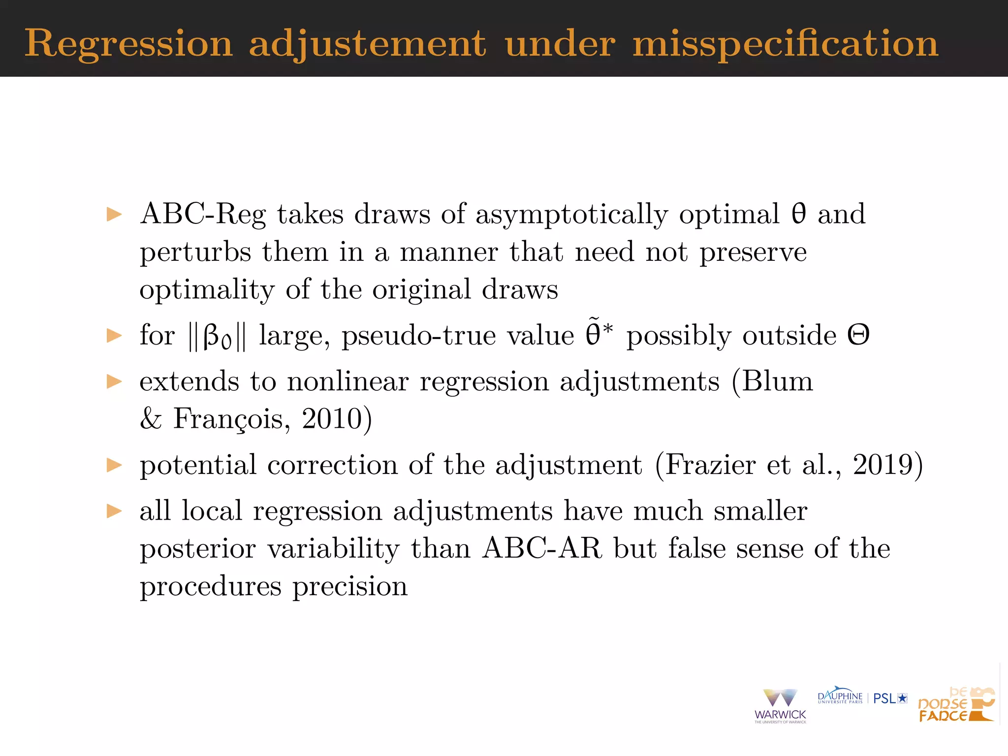
![Regression adjustement under misspecification
Original accepted value θ artificially related to η(xobs) and η(z)
through local linear regression model
θ = µ + β {η(xobs
) − η(z)} + ν,
where νi model residual
[Beaumont et al., 2003]
Asymptotic behavior of ABC-Reg posterior
Πε[·|η(xobs
)]
determined by behavior of
Πε[·|η(xobs
)], ^β, and {η(xobs
) − η(z)}](https://image.slidesharecdn.com/jsm19-190720162758/75/the-ABC-of-ABC-120-2048.jpg)
![Regression adjustement under misspecification
Original accepted value θ artificially related to η(xobs) and η(z)
through local linear regression model
θ = µ + β {η(xobs
) − η(z)} + ν,
where νi model residual
[Beaumont et al., 2003]
Asymptotic behavior of ABC-Reg posterior
Πε[·|η(xobs
)]
determined by behavior of
Πε[·|η(xobs
)], ^β, and {η(xobs
) − η(z)}](https://image.slidesharecdn.com/jsm19-190720162758/75/the-ABC-of-ABC-121-2048.jpg)
![Approximate ABC [AABC]
Idea approximations on both parameter and model spaces by
resorting to bootstrap techniques.
[Buzbas & Rosenberg, 2015]
Procedure scheme
1. Sample (θi, xi), i = 1, . . . , m, from prior predictive
2. Simulate θ∗ ∼ π(·) and assign weight wi to dataset x(i)
simulated under k-closest θi to θ∗ by Epanechnikov kernel
3. Generate dataset x∗ as bootstrap weighted sample from
(x(1), . . . , x(k))
Drawbacks
If m too small, prior predictive sample may miss
informative parameters
large error and misleading representation of true posterior
only well-suited for models with very few parameters](https://image.slidesharecdn.com/jsm19-190720162758/75/the-ABC-of-ABC-127-2048.jpg)
![Approximate ABC [AABC]
Procedure scheme
1. Sample (θi, xi), i = 1, . . . , m, from prior predictive
2. Simulate θ∗ ∼ π(·) and assign weight wi to dataset x(i)
simulated under k-closest θi to θ∗ by Epanechnikov kernel
3. Generate dataset x∗ as bootstrap weighted sample from
(x(1), . . . , x(k))
Drawbacks
If m too small, prior predictive sample may miss
informative parameters
large error and misleading representation of true posterior
only well-suited for models with very few parameters](https://image.slidesharecdn.com/jsm19-190720162758/75/the-ABC-of-ABC-128-2048.jpg)
![Divide-and-conquer perspectives
1. divide the large dataset into smaller batches
2. sample from the batch posterior
3. combine the result to get a sample from the targeted
posterior
Alternative via ABC-EP
[Barthelm´e & Chopin, 2014]](https://image.slidesharecdn.com/jsm19-190720162758/75/the-ABC-of-ABC-129-2048.jpg)
![Divide-and-conquer perspectives
1. divide the large dataset into smaller batches
2. sample from the batch posterior
3. combine the result to get a sample from the targeted
posterior
Alternative via ABC-EP
[Barthelm´e & Chopin, 2014]](https://image.slidesharecdn.com/jsm19-190720162758/75/the-ABC-of-ABC-130-2048.jpg)
![Geometric combination: WASP
Subset posteriors given partition xobs
[1] , . . . , xobs
[B] of the
observed data xobs, let define
π(θ | xobs
[b] ) ∝ π(θ)
j∈[b]
f(xobs
j | θ)B
.
[Srivastava et al., 2015]
Subset posteriors are combined using the Wasserstein
barycenter
[Cuturi, 2014]
Drawback require sampling from f(· | θ)B by ABC means.
Should be feasible for latent variable (z) representations when
f(x | z, θ) available in closed form
[Doucet & Robert, 2001]](https://image.slidesharecdn.com/jsm19-190720162758/75/the-ABC-of-ABC-131-2048.jpg)
![Geometric combination: WASP
Subset posteriors given partition xobs
[1] , . . . , xobs
[B] of the
observed data xobs, let define
π(θ | xobs
[b] ) ∝ π(θ)
j∈[b]
f(xobs
j | θ)B
.
[Srivastava et al., 2015]
Subset posteriors are combined using the Wasserstein
barycenter
[Cuturi, 2014]
Alternative backfeed subset posteriors as priors to other
subsets](https://image.slidesharecdn.com/jsm19-190720162758/75/the-ABC-of-ABC-132-2048.jpg)
![Consensus ABC
Na¨ıve scheme
For each data batch b = 1, . . . , B
1. Sample (θ
[b]
1 , . . . , θ
[b]
n ) from diffused prior
˜π(·) ∝ π(·)1/B
2. Run ABC to sample from batch posterior
^π(· | d(S(xobs
[b] ), S(x[b])) < ε)
3. Compute sample posterior variance Σb
Combine batch posterior approximations
θj =
B
b=1
Σb
−1 B
b=1
Σbθ
[b]
j .
Remark Diffuse prior quite non informative which call for
ABC-MCMC to avoid sampling from ˜π(·).](https://image.slidesharecdn.com/jsm19-190720162758/75/the-ABC-of-ABC-133-2048.jpg)
![Consensus ABC
Na¨ıve scheme
For each data batch b = 1, . . . , B
1. Sample (θ
[b]
1 , . . . , θ
[b]
n ) from diffused prior
˜π(·) ∝ π(·)1/B
2. Run ABC to sample from batch posterior
^π(· | d(S(xobs
[b] ), S(x[b])) < ε)
3. Compute sample posterior variance Σb
Combine batch posterior approximations
θj =
B
b=1
Σb
−1 B
b=1
Σbθ
[b]
j .
Remark Diffuse prior quite non informative which call for
ABC-MCMC to avoid sampling from ˜π(·).](https://image.slidesharecdn.com/jsm19-190720162758/75/the-ABC-of-ABC-134-2048.jpg)
![Big parameter issues
Curse of dimensionality: as dim(Θ) increases
exploration of parameter space gets harder
summary statistic η forced to increase, since at least of
dimension dim(Θ)
Some solutions
adopt more local algorithms like ABC-MCMCM or
ABC-SMC
aim at posterior marginals and approximate joint posterior
by copula
[Li et al., 2016]
run ABC-Gibbs
[Clart´e et al., 2016]](https://image.slidesharecdn.com/jsm19-190720162758/75/the-ABC-of-ABC-135-2048.jpg)
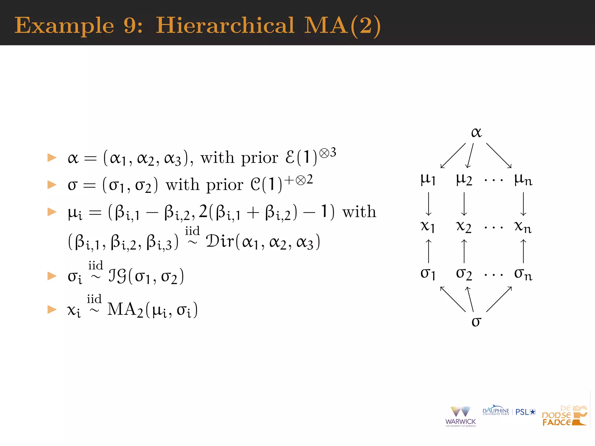
![ABC-Gibbs
When parameter decomposed into θ = (θ1, . . . , θn)
Algorithm 5 ABC-Gibbs sampler
starting point θ(0) = (θ
(0)
1 , . . . , θ
(0)
n ), observation xobs
for i = 1, . . . , N do
for j = 1, . . . , n do
θ
(i)
j ∼ πεj
(· | x , sj, θ
(i)
1 , . . . , θ
(i)
j−1, θ
(i−1)
j+1 , . . . , θ
(i−1)
n )
end for
end for
Divide & conquer:
one tolerance εj for each parameter θj
one statistic sj for each parameter θj
[Clart´e et al., 2016]](https://image.slidesharecdn.com/jsm19-190720162758/75/the-ABC-of-ABC-138-2048.jpg)
![ABC-Gibbs
When parameter decomposed into θ = (θ1, . . . , θn)
Algorithm 6 ABC-Gibbs sampler
starting point θ(0) = (θ
(0)
1 , . . . , θ
(0)
n ), observation xobs
for i = 1, . . . , N do
for j = 1, . . . , n do
θ
(i)
j ∼ πεj
(· | x , sj, θ
(i)
1 , . . . , θ
(i)
j−1, θ
(i−1)
j+1 , . . . , θ
(i−1)
n )
end for
end for
Divide & conquer:
one tolerance εj for each parameter θj
one statistic sj for each parameter θj
[Clart´e et al., 2016]](https://image.slidesharecdn.com/jsm19-190720162758/75/the-ABC-of-ABC-139-2048.jpg)
![Compatibility
When using ABC-Gibbs conditionals with different acceptance
events, e.g., different statistics
π(α)π(sα(µ) | α) and π(µ)f(sµ(x ) | α, µ).
conditionals are incompatible
ABC-Gibbs does not necessarily converge (even for
tolerance equal to zero)
potential limiting distribution
not a genuine posterior (double use of data)
unknown [except for a specific version]
possibly far from genuine posterior(s)
[Clart´e et al., 2016]](https://image.slidesharecdn.com/jsm19-190720162758/75/the-ABC-of-ABC-140-2048.jpg)
![Compatibility
When using ABC-Gibbs conditionals with different acceptance
events, e.g., different statistics
π(α)π(sα(µ) | α) and π(µ)f(sµ(x ) | α, µ).
conditionals are incompatible
ABC-Gibbs does not necessarily converge (even for
tolerance equal to zero)
potential limiting distribution
not a genuine posterior (double use of data)
unknown [except for a specific version]
possibly far from genuine posterior(s)
[Clart´e et al., 2016]](https://image.slidesharecdn.com/jsm19-190720162758/75/the-ABC-of-ABC-141-2048.jpg)
![ABC sessions at JSM [and further]
#107 - The ABC of Making an Impact, Monday
8:30-10:20am
#???
[A]BayesComp, Jan 7-10 2020
ABC in Grenoble, March 18-19 2020
ABC in Longyearbyen, April 8-9 2021](https://image.slidesharecdn.com/jsm19-190720162758/75/the-ABC-of-ABC-144-2048.jpg)
![ABC sessions at JSM [and further]
#107 - The ABC of Making an Impact, Monday
8:30-10:20am
#???
[A]BayesComp, Jan 7-10 2020
ABC in Grenoble, March 18-19 2020
ABC in Longyearbyen, April 8-9 2021](https://image.slidesharecdn.com/jsm19-190720162758/75/the-ABC-of-ABC-145-2048.jpg)

The document describes Approximate Bayesian Computation (ABC), a technique for performing Bayesian inference when the likelihood function is intractable or impossible to evaluate directly. ABC works by simulating data under different parameter values, and accepting simulations that are close to the observed data according to a distance measure and tolerance level. ABC provides an approximation to the posterior distribution that improves as the tolerance level decreases and more informative summary statistics are used. The document discusses the ABC algorithm, properties of the exact ABC posterior distribution, and challenges in selecting appropriate summary statistics.


![Inference in generative models using the Wasserstein distance [[INI]](https://cdn.slidesharecdn.com/ss_thumbnails/inewton-170706120746-thumbnail.jpg?width=640&height=640&fit=bounds)