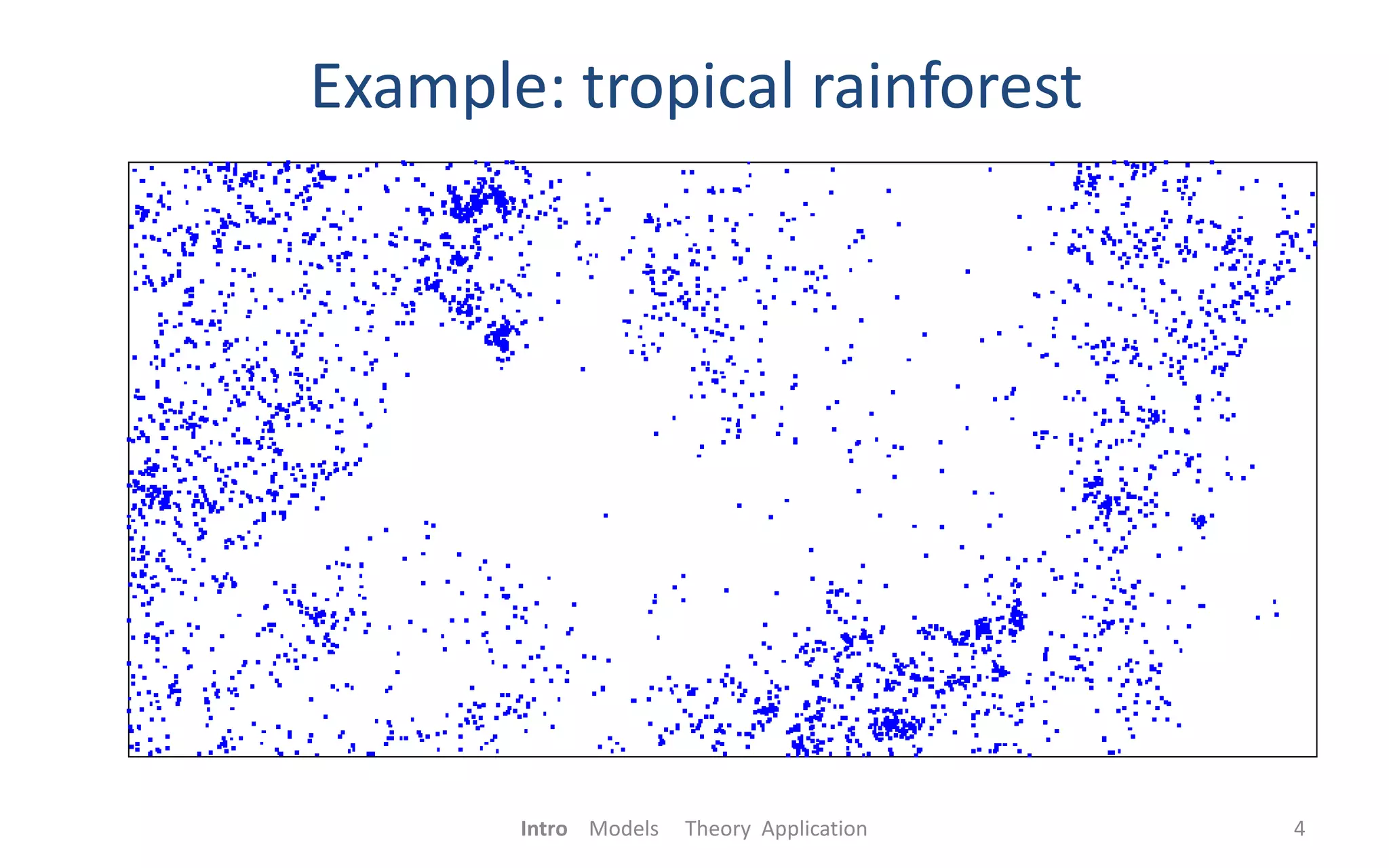
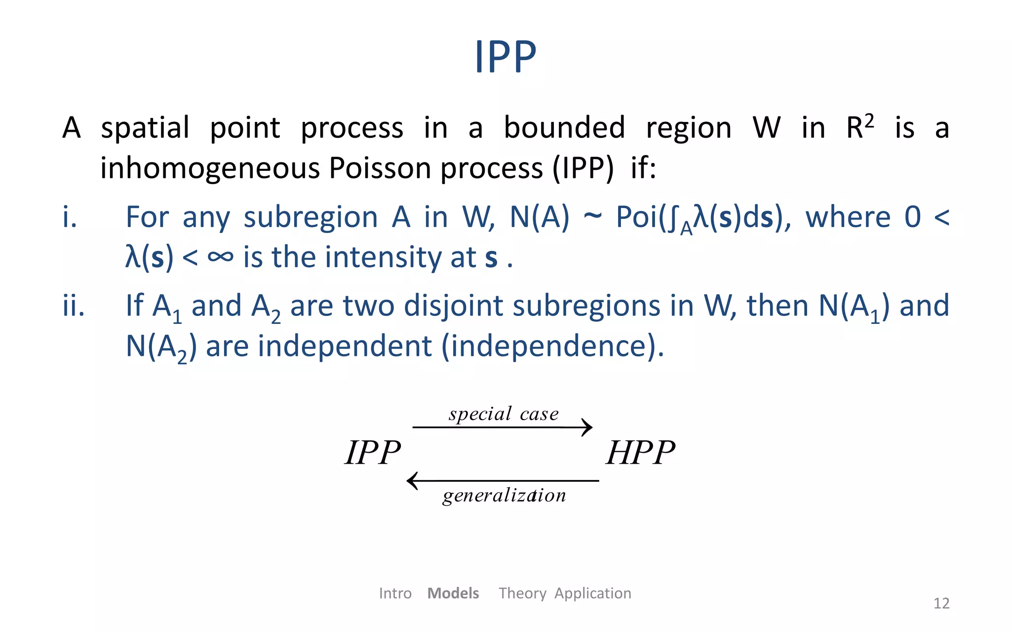
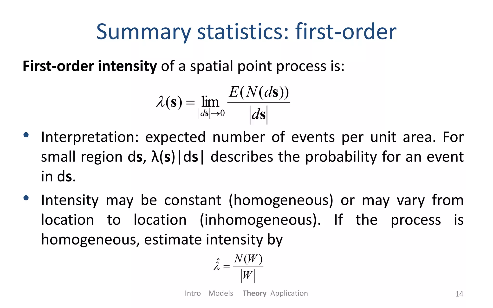
Spatial statistics can be used in epidemiology to analyze spatial point patterns of disease cases and controls. Common models include homogeneous and inhomogeneous Poisson processes, which describe patterns of complete spatial randomness and non-random clustering or dispersion. Descriptive statistics like the first-order intensity function λ(s) and second-order K-function can quantify clustering in a point pattern. A case-control study compares these statistics between case and control patterns to test for non-random spatial variations in disease risk. Monte Carlo simulations are used to calculate p-values when testing hypotheses about relative risk and clustering.

1. Spatial Statistics for Epidemiology
—Spatial Point Processes
By Liu Xu U086105E
Supervisor: Prof Loh Wei Liem
Department of Statistics and Applied Probability
National University of Singapore
15 March 2012
1

2. Outline
Application in epidemiology
Theory: descriptive statistics
Models: spatial point processes
Data: spatial point patterns
2

3. A spatial point pattern is …
Space → Rd, d ≥ 2
Points → data values
Pattern → arrangement
Intro Models Theory Application 3

4. Example: tropical rainforest
Intro Models Theory Application 4

5. Example: cancer cases
Intro Models Theory Application
5
marks: extra information
attached to points,
categorical/ continuous

6. Example : the milky way galaxy
Intro Models Theory Application 6

7. Types of point patterns
Intro Models Theory Application
7
regularityCSRclustering repulsionattraction
  

8. Aim: describe and model “pattern”
Are points randomly located?
• If so, find a statistical model to
describe the “randomness”;
• If not, …
Intro Models Theory Application
8

9. Models: spatial point processes
• A spatial point process is a stochastic process X which
generates a countable set of events in defined space.
• A spatial pattern x = {x1, x2, …, xn} on an observational region
W generated from a spatial point process is a realization of
the process.
• Only consider point processes in 2-D space.
• The locations of any object can be modelled−plants, animals,
cells, stars, disease cases, earthquakes, …
Intro Models Theory Application
9

10. Models: spatial point processes
Intro Models Theory Application
10
• Notation:
W: study region in R2
N(A): number of events inside subregion A, A W.
|A|: area of region A
s: random locations in W
ds: infinitesimal region centered at s
• Assumptions on spatial point processes:
i. Locally finite: the number of events in any bounded region is bounded
ii. At any point location s, there is either one event or no events at all


11. HPP
A spatial point process in a bounded region W in R2 is a
homogeneous Poisson process (HPP) if:
i. For all subregion A in W, N(A) ~ Poi(λ|A|), where 0 < λ < ∞
is a constant, called intensity (homogeneity).
ii. If A1 and A2 are two disjoint subregions in W, then N(A1) and
N(A2) are independent (independence).
• Standard model for complete spatial randomness (CSR);
• Can be generalized to more complicated models;
• A reference process when analyzing spatial characteristics of
a specific pattern.
Intro Models Theory Application
11

12. IPP
A spatial point process in a bounded region W in R2 is a
inhomogeneous Poisson process (IPP) if:
i. For any subregion A in W, N(A) ~ Poi(∫Aλ(s)ds), where 0 <
λ(s) < ∞ is the intensity at s .
ii. If A1 and A2 are two disjoint subregions in W, then N(A1) and
N(A2) are independent (independence).
Intro Models Theory Application
12
HPPIPP
tiongeneraliza
casespecial
 
 

13. Simulation from Poisson processes
Intro Models Theory Application
13
Two Poisson process realizations on the unit square having the same
expected number of events = 100.

14. Summary statistics: first-order
First-order intensity of a spatial point process is:
• Interpretation: expected number of events per unit area. For
small region ds, λ(s)|ds| describes the probability for an event
in ds.
• Intensity may be constant (homogeneous) or may vary from
location to location (inhomogeneous). If the process is
homogeneous, estimate intensity by
Intro Models Theory Application 14
s
s
s
s d
dNE
d
))((
lim)(
0

W
WN )(ˆ 

15. Estimate λ(s) in inhomogeneous case
• Estimating the intensity of a spatial point pattern is similar to estimating a
bivariate probability density
• How to estimate bivariate density?
Given an i.i.d. sample (y1, . . . , yn) of a bivariate random variable Y, an estimate of
the density f (·) of Y at y is
where K(·) is the kernel and h is the bandwidth.
• The expression for kernel smoothing of the intensity function of a point
pattern x = {x1, …, xn} at location s is
the bandwidth h is chosen based on some cross-validation criterion.
Intro Models Theory Application
15



n
i
)
h
K(
nh
)(f
1
2
1ˆ i
yy
y



n
i
)
h
K(
h
)(λ
1
2
1ˆ sx
s i

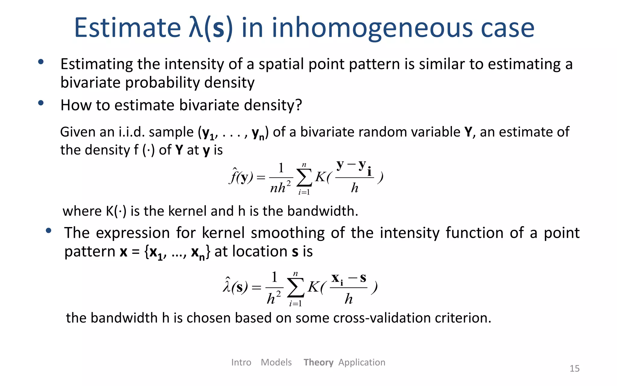
16. Kernel smoothed intensity of IPP
Intro Models Theory Application
16
Kernel estimated intensity for the point pattern simulated from HPP
with λ(s) = 400xy on [0, 1] * [0, 1].

17. Summary statistics: second-order
The second-order properties of a point process involve
relationship between number of events at different locations.
• The second-order intensity of a spatial point process is
• A point process is called stationary if
• A stationary point process is isotropic if
Intro Models Theory Application 17










ji
ji
ss
ji
ss
ss
ss
ji dd
dNdNE
dd
)]()([
lim),(
0,
2





)(),(
,)(
22 jiji ssss
ss


)(),( 22 jiji ssss  

18. If a point process is stationary and isotropic, the K-function of
the process is defined by:
λK(r) = E[number of further events within distance r from an
arbitrary event]
Two properties of K-function:
• For a HPP, λK(r) = λπr2 , thus Kp(r) = πr2
• K(r) is invariant to random thinning.
Intro Models Theory Application
18
K-function
Def. random thinning: each event of a point process X is either
retained or deleted with retention probability p, independently of
other events. The resulting point process X’ contains a subset of
events of the original process X.

19. Comparing estimated K-functions of simulated point patterns
Intro Models Theory Application 19
CSR: K(r) = πr2
clustered: K(r) > πr2
regular: K(r) < πr2

20. Estimation of K(r):Ê(# further events…)/λ̂
Intro Models Theory Application
20
negatively biased edge correction

21. Application in epidemiology
John Snow (15 March 1813 – 16 June
1858) is considered to be one of the
fathers of epidemiology, because of his
work in tracing the source of a cholera
outbreak in Soho, England, in 1854
Intro Models Theory Application
21

22. Case-control study
Goal: compare the spatial distribution
of disease cases with the underlying
population
• Null hypothesis :
equal spatial distribution
• Controls:
selected to represent population
heterogeneity
Intro Models Theory Application
22
Incidence
of disease
Population
density
Overall
risk of
disease
Other risk
factors, e.g.
distance from
point source
Do disease cases occur randomly
among population?

23. Case-control data consist of two point patterns:
• the locations of n1 cases of particular disease {x1, x2, …, xn1}
• the locations n0 controls {xn1+1, …, xn1+n0}
in a study region W over a defined period of time. Total
number of data points n = n1 + n0.
Assumption:
• Cases from an IPP with intensity λ1(s)
• Controls from another independent IPP with intensity λ0(s)
Intro Models Theory Application
23

24. Spatial risk
relative risk:
estimated relative risk:
H0:
test statistic:
estimated test statistic:
significance: Monte Carlo test
Intro Models Theory Application
24
)(
)(
)(
0
1
s
s
s


 
0
1
0)(
n
n
  s


n
i
T
1
2
0 ])([  ix


n
i
T
1
2
0 ])(ˆ[ˆ  ix
)(ˆ
)(ˆ
)(ˆ
0
1
s
s
s


 

25. Spatial clustering
K0(r)→ amount of clustering due to population
K1(r)→ amount of clustering due to population plus effect
of other possible risk factors
D(r) = K1(r) - K0(r) → the amount of clustering that is not
due to population
estimate:
H0:
Test statistic:
significance: Monte Carlo test
Intro Models Theory Application
25


m
k k
k
rD
rD
D
1 )](var[
)(
)(ˆ)(ˆ)(ˆ
01 rKrKrD 
0D(r)=

26. Monte Carlo test
1). simulation with random labelling at jth iteration, j=1, 2, …, 99
• randomly select n1 points from n data points and label the selected points as “case”, label
the remaining n0 points as “control”
• with the relabelled data, estimate kernel smoother and at every data point.
• estimate K1j(r) and K0j(r) and compute D̂j(r) at a set of discrete distances {r1, r2, …, rm} .
2). test statistic
• for each j, compute
• compute the variance of D̂(rk) for each k=1, 2, …, m. then get
3). p-value
Intro Models Theory Application
26
)(ˆ),(ˆ
01 xx jj  )(ˆ xj
2
1 0 ])(ˆ[ˆ 

n
i ijjT  x


m
k
k
kj
j
rD
rD
D
1 )](ˆvar[
)(ˆ
ˆ
)199/(]1}ˆˆ{[
)199/(]1}ˆˆ{[
99
1
2
99
1
1






j
j
j
j
DDIp
TTIp

27. Case study-the chorley data
Intro Models Theory Application
27
58 cases 978 controls

28. Lots of graphs
Intro Models Theory Application
28

29. Intro Models Theory Application
29
Monte Carlo test gives p-value = 0.64 →there is no significant spatial variation in
the relative risk.

30. graph
Intro Models Theory Application
30
p-value = 0.91
→ no significant
relative spatial
clustering

31. Summary
summary 31
Spatial point
patterns
Spatial point
processes
HPP
IPP
λ(s)
K(r)
CSR
Application in
epidemiology

32. Thank you for your attention!
Time for Q&A
The end 32