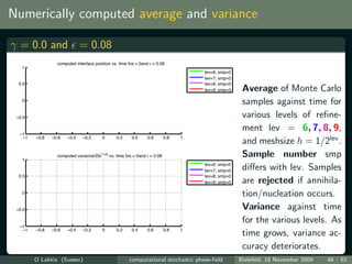
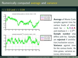
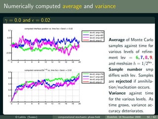
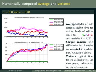
The document discusses computational aspects of stochastic phase-field models. It begins by motivating the inclusion of thermal noise in phase-field simulations through examples of dendrite formation. It then provides background on the deterministic phase-field and Allen-Cahn models before introducing the stochastic Allen-Cahn equation with additive white noise. The remainder of the document discusses the importance of studying this problem both theoretically and computationally, as well as outlining the topics to be covered in more depth.

![Dendrites
Computed dendrites without ther- A computed dendrite with thermal
mal noise [Nestler et al., 2005] noise [Nestler et al., 2005]
O Lakkis (Sussex) computational stochastic phase-field Bielefeld, 18 November 2009 4 / 62](https://image.slidesharecdn.com/091118lakkis3wordsbielefeld-12658912975641-phpapp01/85/computational-stochastic-phase-field-4-320.jpg)
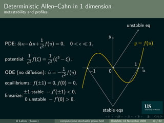
![Deterministic Phase Field
following [Chen, 1994]
Phase transition in solidification process
α ∂t u − ∆u + (u3 − u)/ = σw (“interface” motion)
c∂t w − ∆w = −∂t u (diffusion in bulk) ,
where
≈ 1
solid phase,
u : order parameter/phase field ∈ (−1 + δ , 1 − δ ) , interface (region)
≈ −1 liquid phase.
w : temperature in liquid/solid bulk
O Lakkis (Sussex) computational stochastic phase-field Bielefeld, 18 November 2009 5 / 62](https://image.slidesharecdn.com/091118lakkis3wordsbielefeld-12658912975641-phpapp01/85/computational-stochastic-phase-field-5-320.jpg)

![Why do we care?
about the (deterministic) Allen–Cahn
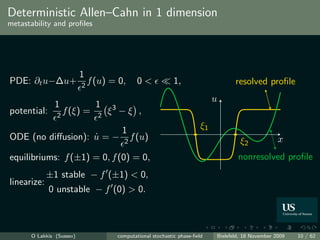
1
∂t u − ∆u + 2
u3 − u = 0
Phase-separation models in metallurgy [Allen and Cahn, 1979].
Simplest model of more complicated class [Cahn and Hilliard, 1958].
Cubic nonlinearity approximation of “harder” (logarithmic) potential.
Double obstacle can replace cubic by other.
Phase-field models of phase separation and geometric motions
[Rubinstein et al., 1989], [Evans et al., 1992], [Chen, 1994],
[de Mottoni and Schatzman, 1995], . . . ;
Metastability, exponentially slow motion in d = 1,
[Carr and Pego, 1989], [Fusco and Hale, 1989],
[Bronsard and Kohn, 1990];
O Lakkis (Sussex) computational stochastic phase-field Bielefeld, 18 November 2009 7 / 62](https://image.slidesharecdn.com/091118lakkis3wordsbielefeld-12658912975641-phpapp01/85/computational-stochastic-phase-field-7-320.jpg)
![Why do we care?
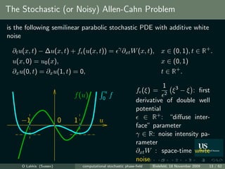
about the stochastic Allen–Cahn
1
∂t u − ∆u + 2
u3 − u = γ
∂xt W
Noise = stabilizing/destabilizing mechanism [Brassesco et al., 1995],
[Funaki, 1995].
Stochastic 1d: Basic existence theory [Faris and Jona-Lasinio, 1982].
Stochastic MCF of interfaces colored space-time/time-only noises
possible [Souganidis and Yip, 2004], [Funaki, 1999],
[Dirr et al., 2001].
Rigorous mathematical setting to noise-induced dendrites.
O Lakkis (Sussex) computational stochastic phase-field Bielefeld, 18 November 2009 8 / 62](https://image.slidesharecdn.com/091118lakkis3wordsbielefeld-12658912975641-phpapp01/85/computational-stochastic-phase-field-8-320.jpg)
![Why do we care?
Modeling and computation with stochastic Allen–Cahn
Stochastic Allen–Cahn (aka Ginzburg–Landau) with noise in materials
science:
Modeling in phenomenological/lattice approximation, noise = unknown
meso/micro-scopic fluctuation with known statistics effect in
macroscopic scale [Halperin and Hoffman, 1977],
[Katsoulakis and Szepessy, 2006, cf.];
Simulation noise as ad-hoc nucleation/instability inducing mechanism
[Warren and Boettinger, 1995, Nestler et al., 2005, e.g.,];
Numerics for d = 1 SDE approach [Shardlow, 2000], spectral methods
[Liu, 2003], interface nucleation/annihilation [Lythe, 1998,
Fatkullin and Vanden-Eijnden, 2004].
Numerics for d ≥ 2 ?
O Lakkis (Sussex) computational stochastic phase-field Bielefeld, 18 November 2009 9 / 62](https://image.slidesharecdn.com/091118lakkis3wordsbielefeld-12658912975641-phpapp01/85/computational-stochastic-phase-field-9-320.jpg)
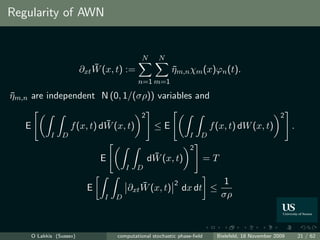
![White noise ∂xt W : an informal definition
Informally: white noise is mixed derivative of (2 dimensional)
Brownian sheet W = Wx,t .
Brownian sheet W : extension of 1-dim Brownian motion to
multi-dim, built on Ω.
Solutions of PDE understood as mild solution
Notation for ∂xt W
∞ 1 ∞ 1
f (x, t) dW (x, t) := f (x, t)∂xt W (x, t) dx dt,
0 0 0 0
stochastic integral [Walsh, 1986].
O Lakkis (Sussex) computational stochastic phase-field Bielefeld, 18 November 2009 14 / 62](https://image.slidesharecdn.com/091118lakkis3wordsbielefeld-12658912975641-phpapp01/85/computational-stochastic-phase-field-15-320.jpg)
![White noise 101
∀A ∈ Borel(R2 ) dW (x, t) =: W (A) ∈ N (0, |A|) , I.e, W (A) is a
A
0-mean Gaussian random variable with variance = |A|.
A ∩ B = ∅ ⇒ W (A),W (B) independent and
W (A ∪ B) = W (A) + W (B).
t x
Brownian sheet: Wx,t = W ([0, t] × [0, x]) = dW (x, t).
0 0
Basic yet crucial property:
2
E f (x, t) dW (x, t) =E f (x, t)2 dx dt , ∀f ∈ L2 .
I D I D
√
(Aka dW = dx dt.)
O Lakkis (Sussex) computational stochastic phase-field Bielefeld, 18 November 2009 15 / 62](https://image.slidesharecdn.com/091118lakkis3wordsbielefeld-12658912975641-phpapp01/85/computational-stochastic-phase-field-16-320.jpg)
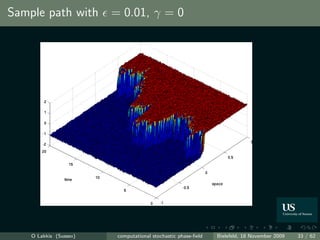
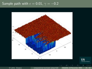
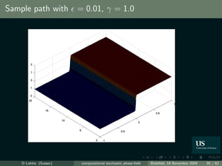
![Solutions of the stochastic Allen–Cahn problem
γ
∂t u(x, t) − ∆u(x, t) + f (u(x, t)) = ∂xt W (x, t), for x ∈ D = [0, 1], t ∈ [0, ∞
u(x, 0) = u0 (x), ∀x ∈ D
∂x u(0, t) = ∂x u(1, t) = 0, ∀t ∈ R+ .
Defined as the continuous solution of integral equation
t
u(x, t) = − Gt−s (x, y)f (u(y, s)) dy ds
0 D
γ
+ Gt (x, y)u0 (y) dy + Zt (x).
D
Unique continuous integral solution exists in 1d provided the initial
condition u0 fulfills boundary conditions.
O Lakkis (Sussex) computational stochastic phase-field Bielefeld, 18 November 2009 17 / 62](https://image.slidesharecdn.com/091118lakkis3wordsbielefeld-12658912975641-phpapp01/85/computational-stochastic-phase-field-18-320.jpg)
![Discretization strategy
In two main steps:
1. Replace white noise ∂xt W by a smoother object: the approximate
¯
white noise ∂xt W .
¯
2. Discretize the approximate problem with ∂xt W via a finite element
scheme for the Allen-Cahn equation.
Inspired by [Allen et al., 1998], [Yan, 2005].
O Lakkis (Sussex) computational stochastic phase-field Bielefeld, 18 November 2009 19 / 62](https://image.slidesharecdn.com/091118lakkis3wordsbielefeld-12658912975641-phpapp01/85/computational-stochastic-phase-field-20-320.jpg)
![Approximate White Noise (AWN)
Fix a final time T > 0 and consider uniform space and time partitions
in space: D = [0, 1], Dm := (xm−1 , xm ), xm − xm−1 = σ, m ∈ [1 : M ] ,
in time: I = [0, T ], In := [tn−1 , tn ), tn − tn−1 = ρ, n ∈ [1 : N ] .
Regularization of the white noise is projection on piecewise constants:
1
ηm,n :=
¯ χm (x)ψn (t) dW (x, t).
σρ I D
N N
¯
∂xt W (x, t) := ηm,n χm (x)ϕn (t).
¯
n=1 m=1
χm = 1Dm , ϕn = 1In (characteristic functions).
O Lakkis (Sussex) computational stochastic phase-field Bielefeld, 18 November 2009 20 / 62](https://image.slidesharecdn.com/091118lakkis3wordsbielefeld-12658912975641-phpapp01/85/computational-stochastic-phase-field-21-320.jpg)
![The regularized problem
∂t u − ∆¯ + f (¯) =
¯ u u γ ¯
∂xt W ,
∂x u(t, 0) = ∂x u(t, 1) = 0,
¯ ¯
u(0) = u0 ,
¯
Admits a “classical” solution. ∀ω ∈ Ω ⇒ corresponding realization of the
¯
AWN ∂xt W (ω) ∈ L∞ ([0, T ] × D) (parabolic regularity) ⇒
∂t u(ω) ∈ L2 ([0, T ]; L2 (D)).
¯
⇒ variational formulation and thus FEM (or other standard methods) now
possible.
Error estimate schedule:
1. Compare u with u.
¯
2. Approximate u by U in a finite element space and compare.
¯
O Lakkis (Sussex) computational stochastic phase-field Bielefeld, 18 November 2009 22 / 62](https://image.slidesharecdn.com/091118lakkis3wordsbielefeld-12658912975641-phpapp01/85/computational-stochastic-phase-field-23-320.jpg)
![The Finite Element Method
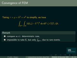
Parameters (numerical mesh) τ, h > 0 (approximation mesh) ρ, σ.
Not necessary, but “natural” coupling: τ = ρ = h2 = σ 2 .
Linearized Semi-Implicit Euler
U n − U n−1
, Φ + ∂x U n , ∂x Φ + f (U n−1 )U n , Φ
τ
= f (U n−1 )U n−1 + f (U n−1 ), Φ + γ ∂xt W , Φ , ∀ Φ ∈ Vh .
¯
Vh is a finite element space of piecewise linear
[Kessler et al., 2004, Feng and Wu, 2005].
O Lakkis (Sussex) computational stochastic phase-field Bielefeld, 18 November 2009 23 / 62](https://image.slidesharecdn.com/091118lakkis3wordsbielefeld-12658912975641-phpapp01/85/computational-stochastic-phase-field-24-320.jpg)
![Maximum principle in probability sense
Lemma
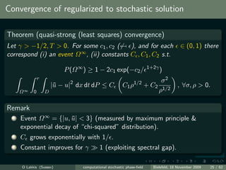
Suppose γ > −1/2. Given T , there exist c1 , c2 , δ0 > 0 such that if
u0 L∞ (D) ≤ 1 + δ0 then
1+2γ
P sup (u, u)(t)
¯ L∞ (D) >3 ≤ c1 exp(−c2 / ).
t∈[0,T ]
Remark
1 The constant 3 is for convenience, can be replaced by 1 + δ1 , if
needed, by adjusting c1 , c2 and δ0 .
2 This result is used to determine the event Ω ∞ for convergence to
hold.
3 Because, nonlinearity is not globally Lipschitz.
O Lakkis (Sussex) computational stochastic phase-field Bielefeld, 18 November 2009 26 / 62](https://image.slidesharecdn.com/091118lakkis3wordsbielefeld-12658912975641-phpapp01/85/computational-stochastic-phase-field-27-320.jpg)
![Small noise resolution (for γ big: weak intensity)
Theorem (small noise)
Let q solution of deterministic the Allen–Cahn problem
∂t q − ∆q + f (q) = 0, q(0) = u0 , on D.
Then ∀ T > 0 : ∃ K1 (T ) > 0, 0 (T ) >0
3
P sup u − q
¯ L2 (D) ≤
[0,T ]
T /(σρ)−1
K1 (T ) 6−2γ K1 (T ) 6−2γ
≥1− 1+ exp −
2 2
for all ∈ (0, 0 ), γ > 3 and ρ, σ > 0.
O Lakkis (Sussex) computational stochastic phase-field Bielefeld, 18 November 2009 27 / 62](https://image.slidesharecdn.com/091118lakkis3wordsbielefeld-12658912975641-phpapp01/85/computational-stochastic-phase-field-28-320.jpg)
![Spectrum estimate
Theorem ([Chen, 1994], [de Mottoni and Schatzman, 1995])
Let q be the (classical) solution of the problem
∂t q − ∆q + f (q) = 0, q(0) = u0 , on D
Key to argument in convergence for weak noise is the use of spectral
estimate for q: There exists a constant λ0 > 0 independent of such that
for any ∈ (0, 1] we have
2 2
∂x φ L2 (D) + f (q)φ, φ ≥ −λ0 φ L2 (D) , ∀φ H1 (D).
O Lakkis (Sussex) computational stochastic phase-field Bielefeld, 18 November 2009 28 / 62](https://image.slidesharecdn.com/091118lakkis3wordsbielefeld-12658912975641-phpapp01/85/computational-stochastic-phase-field-29-320.jpg)
![X(0, T ; L2 (D)) bounds for AWN
Lemma
∀K > 0
P sup ¯
∂xt W (t) ≤K
L2 (D)
t∈[0,T ]
1/(2σ)−1 +
T K2 K2
≥ 1− 1+ ρ exp − ρ
ρ 2 2
T
¯ 2
and P ∂xt W (t) L2 (D)
≤ K2
0
1/(2ρσ)−1
K2 K2
≥1− 1+ exp −
2 2
O Lakkis (Sussex) computational stochastic phase-field Bielefeld, 18 November 2009 29 / 62](https://image.slidesharecdn.com/091118lakkis3wordsbielefeld-12658912975641-phpapp01/85/computational-stochastic-phase-field-30-320.jpg)
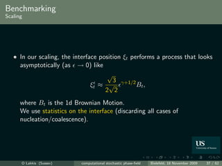
![How to the benchmark our computations?
Benchmarking = “comparing with known solutions” Very few known
“exact result”.
Theorem ( [Funaki, 1995, Brassesco et al., 1995])
The interface motion is asymptotically, as → 0, a (1d) Brownian motion,
lim P sup ˜ ˜
ut − q(x − ξt ) >δ = 0,
→0 t≤ −1−2γ T L2 (D)
for δ > 0.
Remark
q is an instanton for the deterministic Allen-Cahn equation
˜
ξt solves a SODE representing the motion of the interface
ut (x) is an appropriate rescaling of u(x, t).
˜
O Lakkis (Sussex) computational stochastic phase-field Bielefeld, 18 November 2009 36 / 62](https://image.slidesharecdn.com/091118lakkis3wordsbielefeld-12658912975641-phpapp01/85/computational-stochastic-phase-field-37-320.jpg)
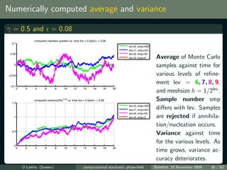
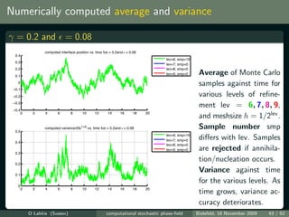
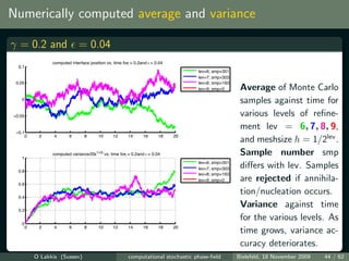
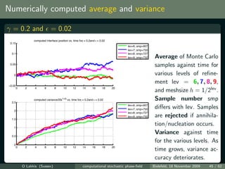
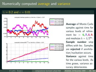
![Simulations vs. theory
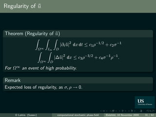
log(var[Uh ] /ti ) vs. log plot for γ = 0.5 at various times ti = t0 10i
i
log(ε)−log(σ(t)2/t) and log(ε)*(1+2*γ) for γ=0.5
−2
ref. slope=1+2*γ
time 0.00152587
−3 time 0.0152587
time 0.152587
time 1.52587
time 15.2587
−4
−5 Theoretical slope
(predicted by
−6
[Funaki, 1995] and
−7 [Brassesco et al., 1995])
is 1 + 2γ.
−8
Plotted in orange refer-
−9 ence line
As → 0 slope im-
−10
−5 −4.5 −4 −3.5 −3 −2.5
proves.
Meshsize h = 1/512.
O Lakkis (Sussex) computational stochastic phase-field Bielefeld, 18 November 2009 42 / 62](https://image.slidesharecdn.com/091118lakkis3wordsbielefeld-12658912975641-phpapp01/85/computational-stochastic-phase-field-43-320.jpg)
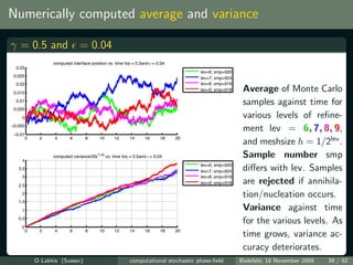
![Simulations vs. theory
log(var[Uh ] /ti ) vs. log plot for γ = 0.2 at various times ti = t0 10i
i
log(ε)−log(σ(t)2/t) and log(ε)*(1+2*γ) for γ=0.2
0
ref. slope=1+2*γ
time 0.00152587
time 0.0152587
−1 time 0.152587
time 1.52587
time 15.2587
−2
Theoretical slope
−3
(predicted by
−4
[Funaki, 1995] and
[Brassesco et al., 1995])
−5 is 1 + 2γ.
Plotted in orange refer-
−6
ence line
As → 0 slope im-
−7
−5 −4.5 −4 −3.5 −3 −2.5
proves.
Meshsize h = 1/512.
O Lakkis (Sussex) computational stochastic phase-field Bielefeld, 18 November 2009 47 / 62](https://image.slidesharecdn.com/091118lakkis3wordsbielefeld-12658912975641-phpapp01/85/computational-stochastic-phase-field-48-320.jpg)
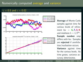
![Simulations vs. theory
log(var[Uh ] /ti ) vs. log plot for γ = 0.0 at various times ti = t0 10i
i
log(ε)−log(σ(t)2/t) and log(ε)*(1+2*γ) for γ=0
0
ref. slope=1+2*γ
time 0.00152587
−0.5
time 0.0152587
time 0.152587
−1 time 1.52587
time 15.2587
−1.5
−2
Theoretical slope
(predicted by
−2.5
[Funaki, 1995] and
−3
[Brassesco et al., 1995])
−3.5
is 1 + 2γ.
−4 Plotted in orange refer-
−4.5
ence line
As → 0 slope im-
−5
−5 −4.5 −4 −3.5 −3 −2.5
proves.
Meshsize h = 1/512.
O Lakkis (Sussex) computational stochastic phase-field Bielefeld, 18 November 2009 52 / 62](https://image.slidesharecdn.com/091118lakkis3wordsbielefeld-12658912975641-phpapp01/85/computational-stochastic-phase-field-53-320.jpg)
![What we’re trying to learn
Current investigation [Kossioris et al., 2009]
finite “exact” solutions
multiple interface convergence
structure of the stochastic solution
colored noise in d > 1
adaptivity
O Lakkis (Sussex) computational stochastic phase-field Bielefeld, 18 November 2009 54 / 62](https://image.slidesharecdn.com/091118lakkis3wordsbielefeld-12658912975641-phpapp01/85/computational-stochastic-phase-field-55-320.jpg)


![[Vvedensky d.] group_theory,_problems_and_solution(book_fi.org)](https://cdn.slidesharecdn.com/ss_thumbnails/vvedenskyd-grouptheoryproblemsandsolutionbookfi-org-130405071812-phpapp02-thumbnail.jpg?width=640&height=640&fit=bounds)