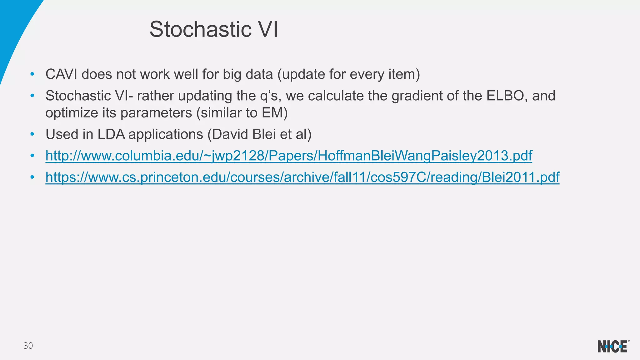
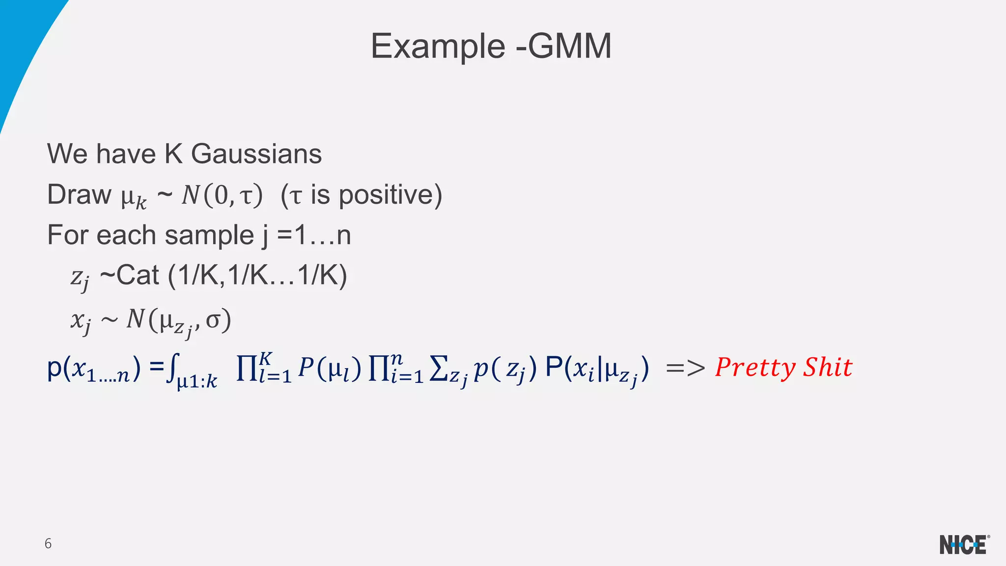
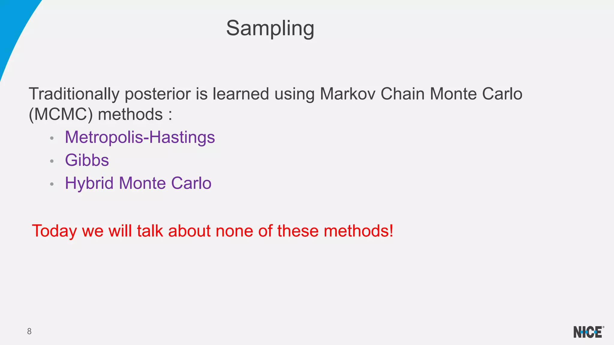
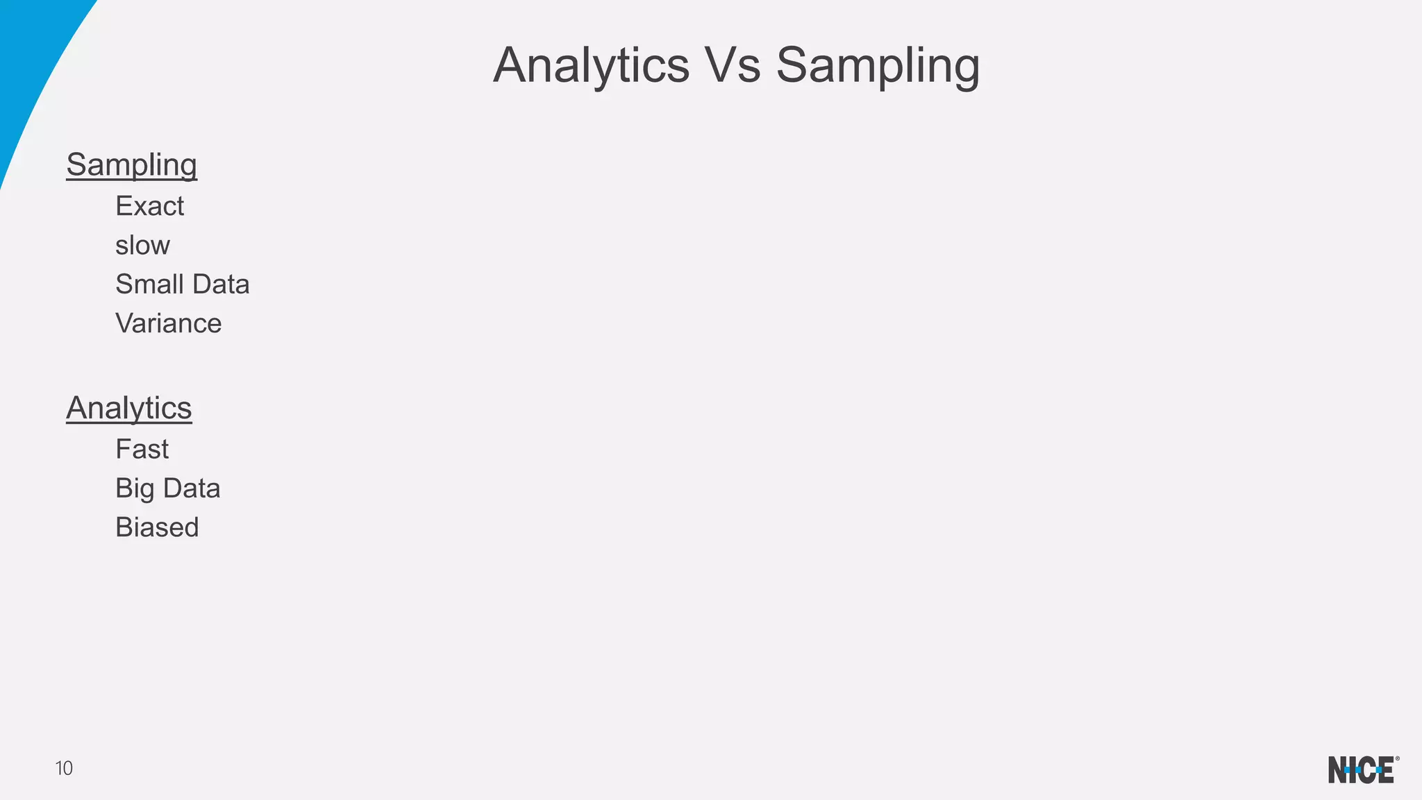
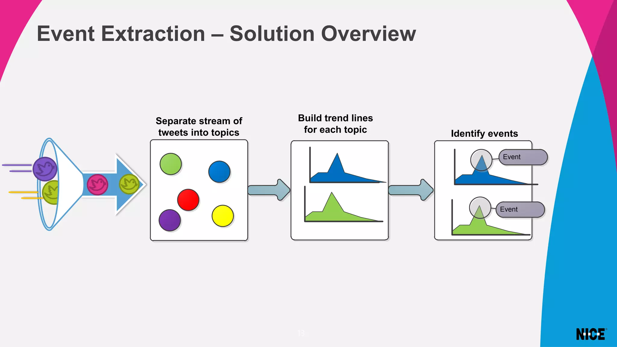
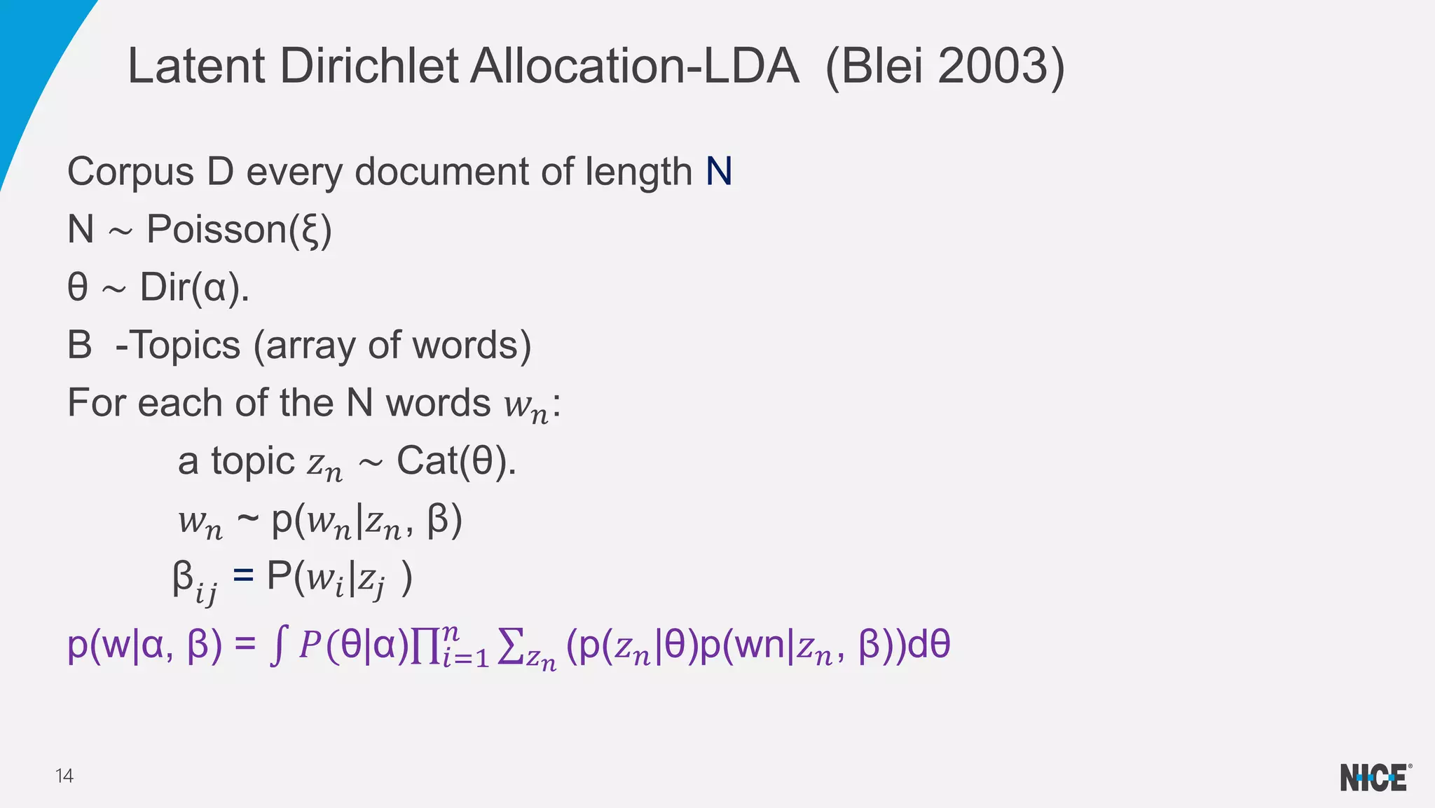
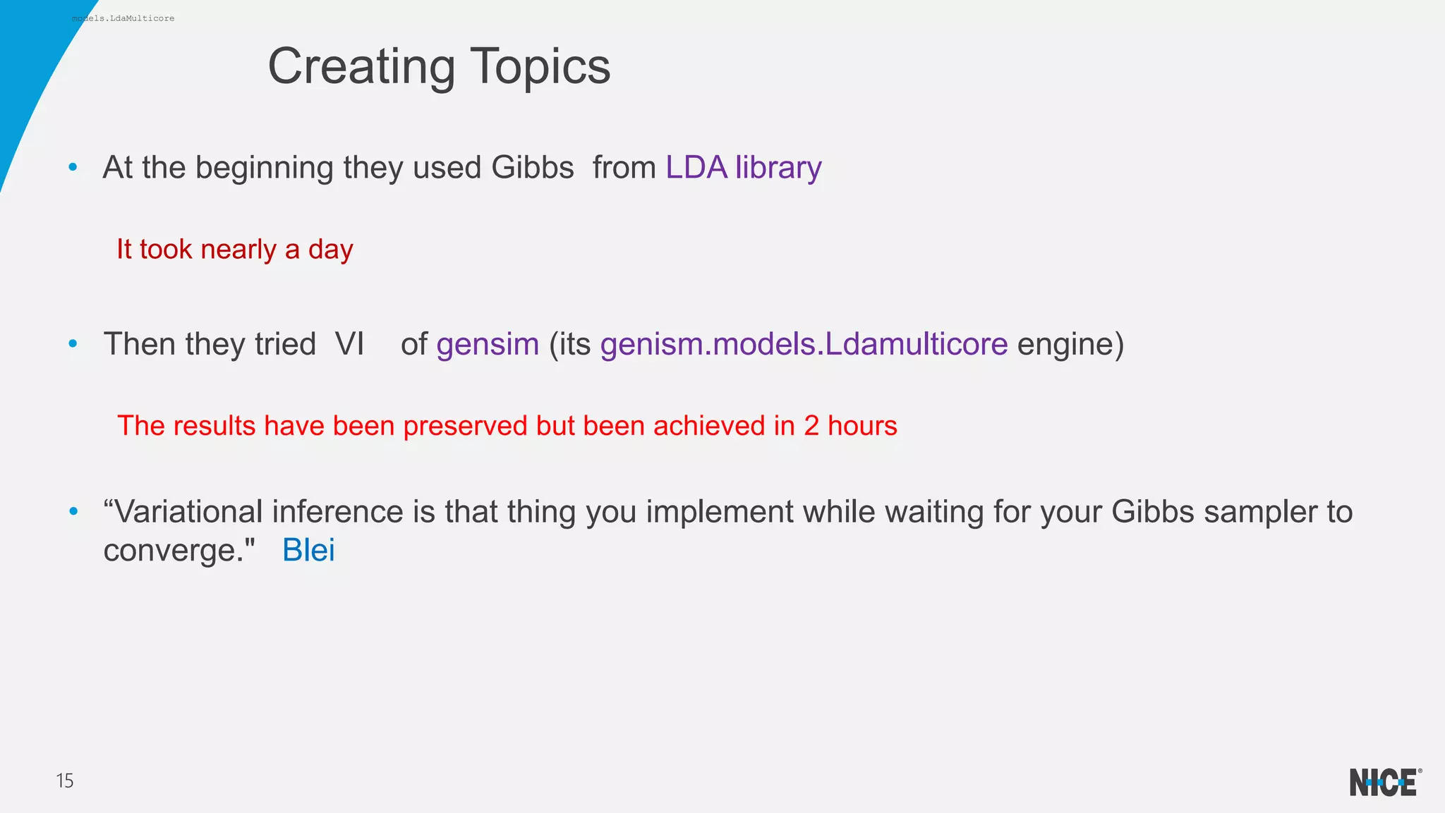
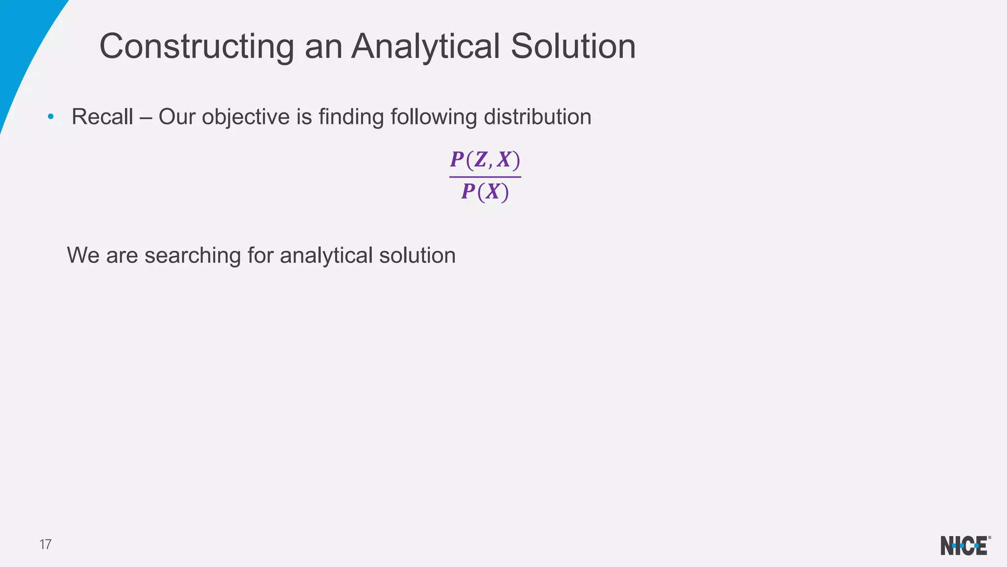
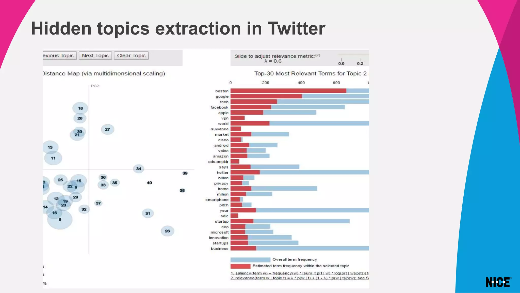
Variational inference is a technique for approximating intractable distributions by optimizing a tractable variational distribution. It was used by Infomedia to identify global events from Twitter data by separating tweets into topics using latent Dirichlet allocation (LDA). Initially Gibbs sampling for LDA took nearly a day but variational inference using Gensim's LDA model converged much faster in 2 hours. Variational inference works by choosing a family of distributions and minimizing the Kullback-Leibler divergence between the true posterior and the variational distribution. This can be done using coordinate ascent variational inference or stochastic variational inference for large datasets.

1. Variational Inference
Natan Katz
Raanana AI
06/01/2020

2. What is Bayesian Inference?
Sampling
When NICE met VI
Rigorous Foundation
Two words on Numeric

3. WHAT IS
BAYESIAN
INFERENCE?

4. Bayesian Inference -Notations
4
The inputs:
Evidence – The Sample of length n (numbers, categories, vectors, images)
Hypothesis - An assumption about the prob. structure that creates the sample
Objective :
We wish to learn the conditional distribution of Hypothesis given the Evidence.
This probability is called Posterior or in mathematical terms P(H|E)

5. Z- R.V. that represents the hypothesis
X- R.V. that represents the evidence
Bayes formula:
P(Z|X) =
𝑷(𝒁,𝑿)
𝑷(𝑿)
Bayesian inference is therefore about working with the RHS terms.
In some case studying the denominator is intractable or extremely difficult
to calculate.
Let’s Formulate
5

6. We have K Gaussians
Draw μ 𝑘 ~ 𝑁 0, τ (τ is positive)
For each sample j =1…n
𝑧𝑗 ~Cat (1/K,1/K…1/K)
𝑥𝑗 ~ 𝑁(μ 𝑧 𝑗
, σ)
p(𝑥1….𝑛) = μ1:𝑘 𝑙=1
𝐾
𝑃(μ𝑙) 𝑖=1
𝑛
𝑧 𝑗
𝑝( 𝑧𝑗) P(𝑥𝑖|μ 𝑧 𝑗
) => 𝑃𝑟𝑒𝑡𝑡𝑦 𝑆ℎ𝑖𝑡
Example -GMM
6

7. SAMPLING

8. Traditionally posterior is learned using Markov Chain Monte Carlo
(MCMC) methods :
• Metropolis-Hastings
• Gibbs
• Hybrid Monte Carlo
Today we will talk about none of these methods!
Sampling
8

9. “AN INTRODUCTION TO VARIATIONAL METHODS FOR GRAPHICAL MODELS”
9

10. Sampling
Exact
slow
Small Data
Variance
Analytics
Fast
Big Data
Biased
Analytics Vs Sampling
10

11. WHEN
NICE
MET
VI

12. • 2017- Innovation authority project on a content traffic in networks
• Their objective was identifying global events by observing twits and
classifying them according to calculated topics.
Infomedia - Global Events
12

13. Event Extraction – Solution Overview
13
Separate stream of
tweets into topics
Build trend lines
for each topic Identify events
Event
Event

14. Corpus D every document of length N
N ∼ Poisson(ξ)
θ ∼ Dir(α).
Β -Topics (array of words)
For each of the N words 𝑤 𝑛:
a topic 𝑧 𝑛 ∼ Cat(θ).
𝑤 𝑛 ~ p(𝑤 𝑛|𝑧 𝑛, β)
β𝑖𝑗 = P(𝑤𝑖|𝑧𝑗 )
p(w|α, β) = 𝑃(θ|α) 𝑖=1
𝑛
𝑧 𝑛
(p(𝑧 𝑛|θ)p(wn|𝑧 𝑛, β))dθ
Latent Dirichlet Allocation-LDA (Blei 2003)
14

15. • At the beginning they used Gibbs from LDA library
It took nearly a day
• Then they tried VI of gensim (its genism.models.Ldamulticore engine)
The results have been preserved but been achieved in 2 hours
• “Variational inference is that thing you implement while waiting for your Gibbs sampler to
converge." Blei
Creating Topics
15
models.LdaMulticore

16. VARIATIONAL-INFERENCE
NERDS’ TIME

17. • Recall – Our objective is finding following distribution
𝑷(𝒁, 𝑿)
𝑷(𝑿)
We are searching for analytical solution
Constructing an Analytical Solution
17

18. What is needed in order to construct such a solution?
1.Being familiar with the frame work
2. Having a metric function over this space
3.Having an optimization methodology
Clause 1 is obvious : we are interested in distribution functions space
Constructing an Analytical Solution (cont)
18

19. • A domain in Math that is analog to calculus of functionals & functions space
Euler-Lagrange eq.
𝐹, 𝑦 functions-(with all the “extras”) and J functional
J(y)= 𝐹( 𝑦, 𝑦′
, 𝑡)𝑑𝑡 (𝑦 𝑖𝑠 𝑑𝑖𝑓𝑓. )
If y is an extremum of J it satisfies Euler-Lagrange eq.
𝑑𝐹
𝑑𝑦
-
𝑑
𝑑𝑡
(
𝑑𝐹
𝑑𝑦′
) = 0
• So we have an optimization….
Calculus of Variations
Euler –Lagrange
19

20. • A metric on distributions “On Information and Sufficiency” 1951 (Ann Math Statist)
Let P,Q distributions :
KL(P||Q) = 𝐸 𝑃 log
𝑃
𝑄
Major Properties:
1. Non-symmetric (It actually measures a subjective distance according to P
2. Positive where 0 is obtained only for KL(P,P)
(proof by concavity of log Lagrange multipliers))
KL Divergence
20

21. Cross Entropy
(P,Q)= H(P)+ KL(P||Q)
PMI Pointwise mutual information
• Let X,Y random variables
• PMI(X,Y)=Log[
𝑃(𝑋=𝑎,𝑌=𝑏)
𝑃 𝑋=𝑎 𝑃(𝑌=𝑏)
]
• KL(P(X/Y=a)||Q(x)) = 𝑥 𝑃(𝑋 = 𝑥|𝑌 = 𝑎)PMI(X=x, Y=a)
KL- Applications
21

22. Can we approximate P(Z|X)?
min KL(Q(z)|| P(Z|X))
We have:
log(P(X)) = 𝐸 𝑄 [log P(x, Z)] − 𝐸 𝑄 [log Q(Z)] + KL(Q(Z)||P(Z|X))
ELBO-Evidence Lower Bound
Remarks
1. LHS is indecent on Z
2. log(P(X)) ≥ ELBO (log concavity)
Hence: Maximizing ELBO =>minimizing KL
VI -Let’s Develop
22

23. 𝐸𝐿𝐵𝑂 = 𝐸 𝑄[log P(X, Z)] − 𝐸 𝑄 [log Q(Z)] = 𝑄𝐿𝑜𝑔(
𝑃(𝑋,𝑍)
𝑄(𝑍)
)= J(Q)
Q may have enormous number of variables, can we do more?
VI Development
23

24. H (σ) = -h 𝑥 𝜎𝑥 − 𝑗 𝑦𝑥 𝜎𝑥 𝜎 𝑦 𝜎 𝑦 ∈ {-1, 1}
Using non correlation assumption, we can the equation becomes
H (σ) = -h 𝑥 𝜎𝑥 − 𝑗𝜎𝑥 𝑥 𝜎 𝑦
The we can replace for each term the sum by the mean off its neighbors
H (σ) = 𝐸0 -μ 𝑥 𝜎𝑥
The solution single Bolzman spin dist.:
P(𝑠𝑖) = 𝑒 𝑎∗𝑠 𝑖 /(𝑒 𝑎∗𝑠 𝑖 +𝑒−𝑎∗𝑠 𝑖)
Isig Model - MFT
24

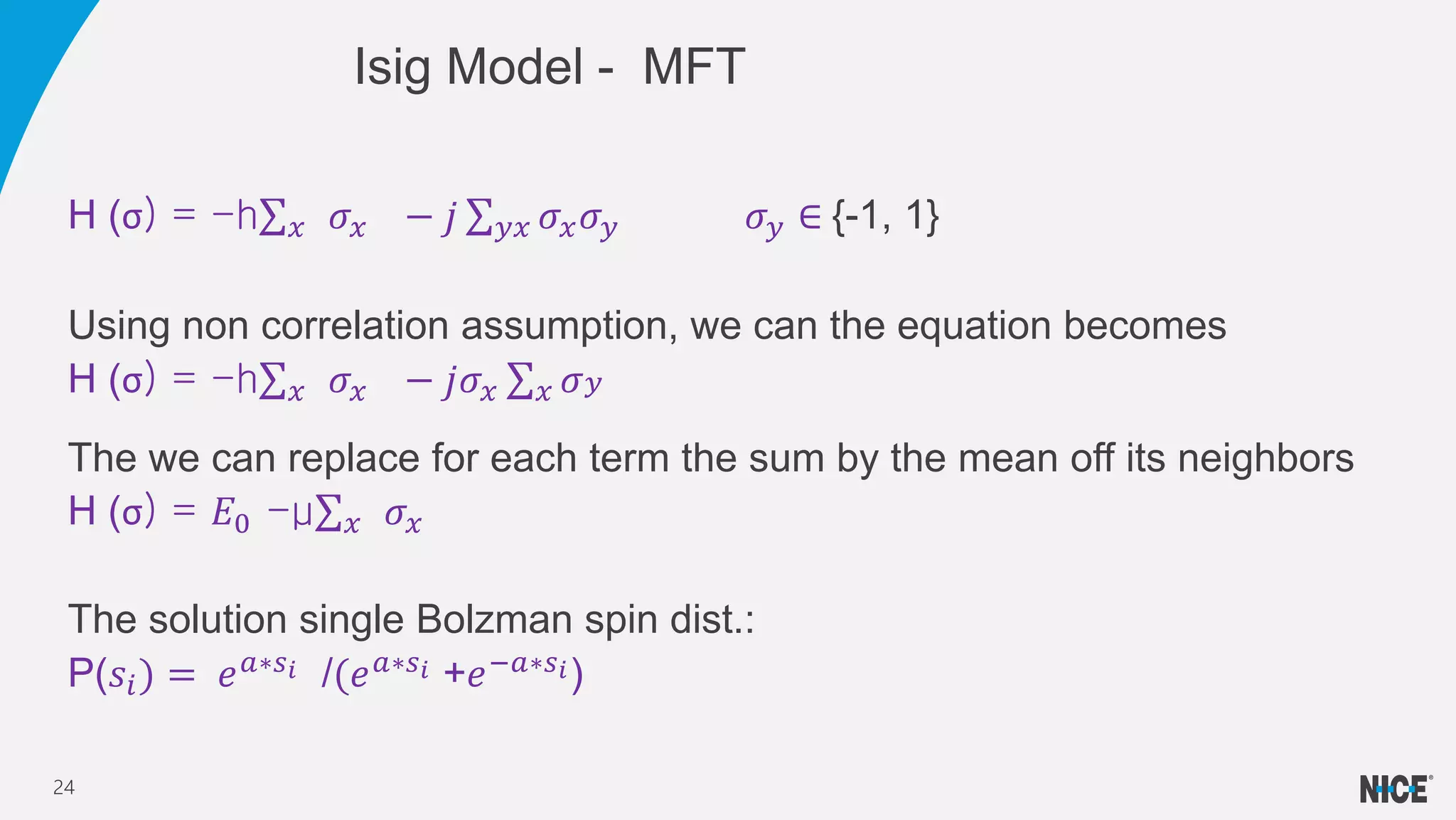
25. • If if Ising & Lenz can do it .why don’t we?
• We assume independency rather non-correlation
𝐸𝐿𝐵𝑂 = 𝐸 𝑄[log P(X, Z)] − 𝐸 𝑄 [log Q(Z)]
Q becomes Q(z) = 𝑖=1
𝑛
𝑞𝑖(𝑧𝑖) (Obviously not true)
• We can use now Euler –Lagrange with the constrain
𝑞𝑖(z) =1
L𝑜𝑔(𝑞𝑖) = 𝑐𝑜𝑛𝑠𝑡 + 𝐸−𝑖[𝑝 𝑥, 𝑧 ] Bolzman Dist.! (as said . We are as good as Ising)
Back to VI
25

26. Hidden topics extraction in Twitter
26

27. NUMERIC

28. • Blei 2018 VI- A review for statistics
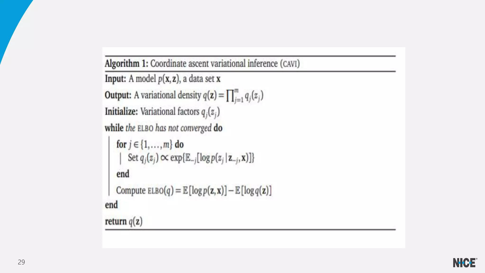
The basic step is set sequentially each 𝑞𝑖 to 𝐸−𝑖[𝑝 𝑥, 𝑧 ] +constant
No 𝑖 𝑡ℎ
coordinate in the RHS (Independency)
Simply update each q until a convergence of ELBO
Coordinate Ascent Variational Inference
CAVI
28

29. 29

30. • CAVI does not work well for big data (update for every item)
• Stochastic VI- rather updating the q’s, we calculate the gradient of the ELBO, and
optimize its parameters (similar to EM)
• Used in LDA applications (David Blei et al)
• http://www.columbia.edu/~jwp2128/Papers/HoffmanBleiWangPaisley2013.pdf
• https://www.cs.princeton.edu/courses/archive/fall11/cos597C/reading/Blei2011.pdf
Stochastic VI
30

31. 31