
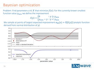
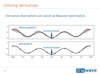
![5
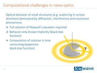
+ Accurate and data
efficient
+ Reliable (provides
uncertainties)
+ Interpretable results
‒ Computationally
demanding but not as
much as training neural
networks
Regression models (small selection)
K-nearest neighbors
Linear regression
Support vector machine
Random forest trees
Gaussian process
regression (Kriging)
(Deep) neural networks
[CE Rasmussen, “Gaussian processes in machine learning”. Advanced lectures on machine
learning , Springer (2004)]
[B. Shahriari et al., "Taking the Human Out of the Loop: A Review of Bayesian Optimization“.
Proc. IEEE 104(1), 148 (2016)]
Increasingpredictivepower
andcomputationaldemands](https://image.slidesharecdn.com/jcmwaveoptimzecompiled-190622220529/85/A-machine-learning-method-for-efficient-design-optimization-in-nano-optics-5-320.jpg)
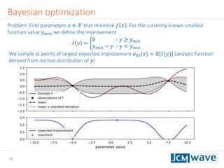
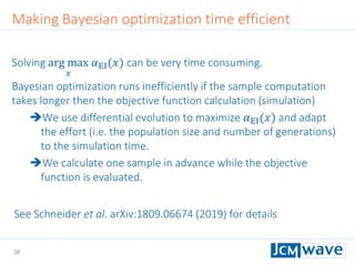
![7
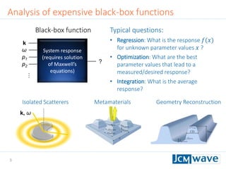
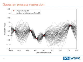
Gaussian process (GP): distribution of functions in a continuous domain 𝒳 ⊂ ℝN
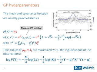
Defined by: mean function 𝜇: 𝒳 → ℝ and covariance function (kernel) 𝑘: 𝒳 × 𝒳 → ℝ
Training data: 𝑀 known function values 𝑓 𝑥1 , … , 𝑓 𝑥 𝑀 with corresponding
covariance matrix 𝐊 = 𝑘 𝑥𝑖, 𝑥𝑗 𝑖,𝑗
Random function values at positions 𝐗∗
= (𝑥1
∗
, … , 𝑥 𝑁
∗
):
Multivariate Gaussian random variable 𝐘∗
∼ 𝒩 𝛍, 𝚺 with probability density
𝑝 𝐘∗
=
1
2𝜋 𝑁/2 𝚺 1/2
exp −
1
2
𝐘∗
− 𝛍 𝑇
𝚺−1
𝐘∗
− 𝛍 ,
means, and covariance
𝛍𝑖 = 𝜇(𝑥𝑖
∗
) −
𝑘𝑙
𝑘 𝑥𝑖
∗
, 𝑥 𝑘 𝐊 𝑘𝑙
−1
[𝑓 𝑥𝑙 − 𝜇 𝑥𝑙 ]
𝚺𝑖𝑗 = 𝑘 𝑥𝑖
∗
, 𝑥𝑗
∗
−
𝑘𝑙
𝑘 𝑥𝑖
∗
, 𝑥 𝑘 𝐊 𝑘𝑙
−1
𝑘 𝑥𝑙, 𝑥𝑗
∗
.
For a proof see:
http://fourier.eng.hmc.edu/e161/lectures/gaussianprocess/node7.html
Gaussian process regression](https://image.slidesharecdn.com/jcmwaveoptimzecompiled-190622220529/85/A-machine-learning-method-for-efficient-design-optimization-in-nano-optics-7-320.jpg)
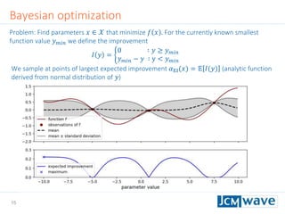
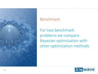
![9
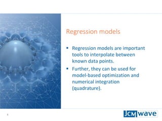
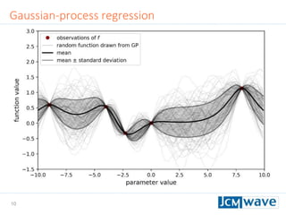
In the following we don’t need correlated random vectors of
function values, but just the probability distribution of a
single function value 𝑦 at some 𝑥∗
∈ 𝒳
This is simply a normal distribution 𝑦 ∼ 𝒩( 𝑦, 𝜎2
) with mean
and standard deviation
𝑦 = 𝜇 𝑥∗ +
𝑖𝑗
𝑘 𝑥∗, 𝑥𝑖 𝐊 𝑖𝑗
−1
[𝑓 𝑥𝑗 − 𝜇 𝑥𝑗 ]
𝜎2 = 𝑘 𝑥∗, 𝑥∗ − 𝑖𝑗 𝑘(𝑥∗, 𝑥𝑖) 𝐊 𝑖𝑗
−1
𝑘(𝑥𝑗, 𝑥∗)
Gaussian process regression](https://image.slidesharecdn.com/jcmwaveoptimzecompiled-190622220529/85/A-machine-learning-method-for-efficient-design-optimization-in-nano-optics-9-320.jpg)
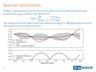
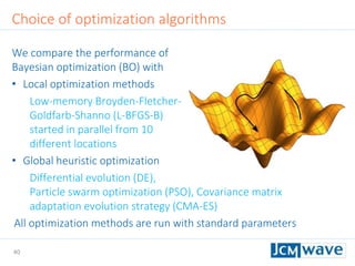
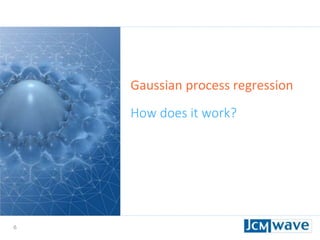
![42
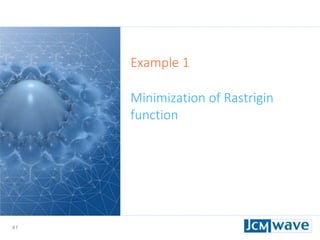
Rastrigin function
Defined on an 𝑛-dimensional domain as 𝑓 𝒙 = 𝐴𝑛 + 𝑖=1
𝑛
[𝑥𝑖
2
− 𝐴 cos(2𝜋𝑥𝑖)] with
𝐴 = 10. We use 𝑛 = 3 and 𝑥𝑖 ∈ [−2.5,2.5].
Sleeping for 10s during evaluation to make function call “expensive”.
Parallel minimization with 5 parallel evaluations of 𝑓 𝒙 .
Global minimum 𝑓 𝑚𝑖𝑛 = 0 at 𝒙 = 0](https://image.slidesharecdn.com/jcmwaveoptimzecompiled-190622220529/85/A-machine-learning-method-for-efficient-design-optimization-in-nano-optics-42-320.jpg)
![43
Benchmark on Rastrigin function
[Laptop with 2-core Intel Core I7 @ 2.7 GHz]
BO converges significantely faster to the global minimum
Derivative observations improve the convergence
Although more elaborate, BO has no significant computation time
overhead](https://image.slidesharecdn.com/jcmwaveoptimzecompiled-190622220529/85/A-machine-learning-method-for-efficient-design-optimization-in-nano-optics-43-320.jpg)
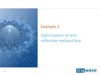
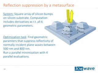
![46
Reflection suppression by a metasurface
Comparison of different global optimization methods
BO more efficient by almost 1 order of magnitude
BO has negligible computation time overhead
[four 10-core Intel Xeon CPUs @ 2.4 GHz]](https://image.slidesharecdn.com/jcmwaveoptimzecompiled-190622220529/85/A-machine-learning-method-for-efficient-design-optimization-in-nano-optics-46-320.jpg)


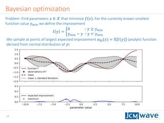
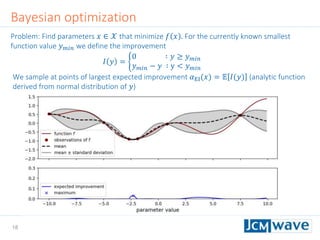
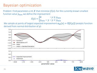
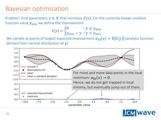
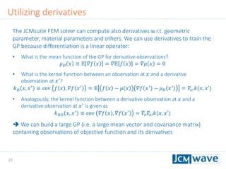
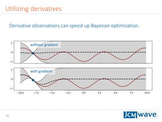
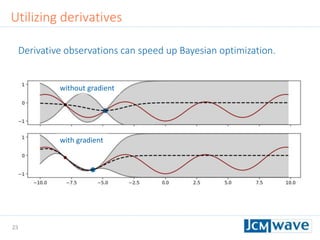
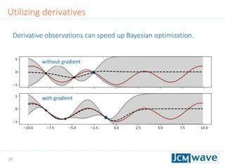
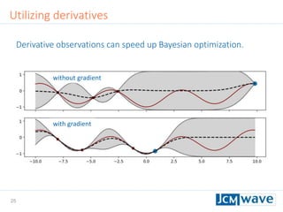
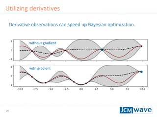
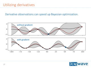
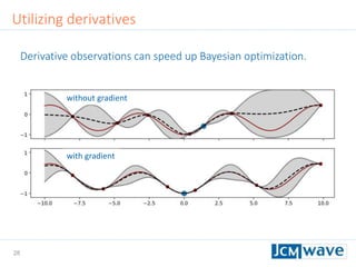
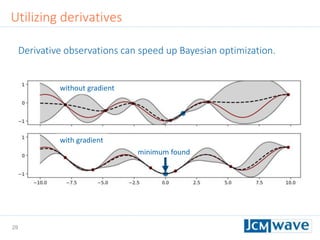
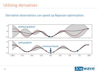
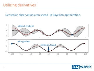
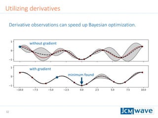
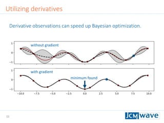
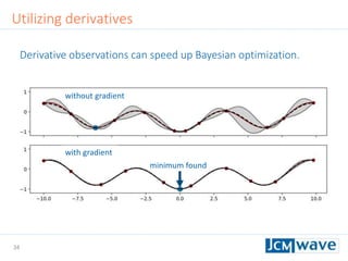
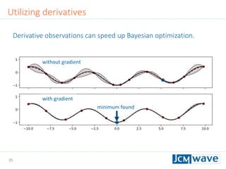
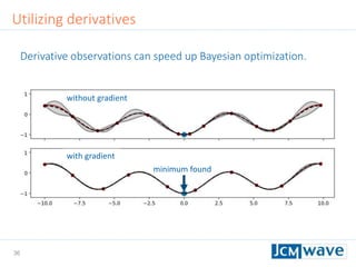
The document describes a machine learning method for efficient design optimization in nano-optics using Gaussian process regression and Bayesian optimization. It discusses how Gaussian process regression can be used to build regression models from expensive black-box functions to enable model-based optimization and integration. Bayesian optimization is then used to iteratively query the black-box function at points of maximum expected improvement to find its minimum. The method can incorporate derivative observations to speed up optimization by providing additional training data for the Gaussian process. Differential evolution is also utilized to efficiently maximize the expected improvement at each iteration. The approach is demonstrated on benchmark optimization problems, showing it outperforms other algorithms like L-BFGS and particle swarm optimization.


![[M2A2] Data Analysis and Interpretation Specialization](https://cdn.slidesharecdn.com/ss_thumbnails/m2a2assigment-170630043040-thumbnail.jpg?width=640&height=640&fit=bounds)


![[DSC Europe 25] Bojan Djuricic - Predictive Design Process.pdf](https://cdn.slidesharecdn.com/ss_thumbnails/5awdrbedqdek3gqu2ezy-4-the-predictive-design-bojan-djuricic-260120105856-6c399e9b-thumbnail.jpg?width=640&height=640&fit=bounds)

![[DSC Europe 25] Mikhail Rozhkov - AI Product Canvas: From Business Goals to T...](https://cdn.slidesharecdn.com/ss_thumbnails/d53doddtpgfqivmzqel6-mikhail-rozhkov-ai-product-canvas-v1-260121115910-9dd517a7-thumbnail.jpg?width=640&height=640&fit=bounds)
![[DSC Europe 25] Borko Kozomora - Optimizing business workflows with advances ...](https://cdn.slidesharecdn.com/ss_thumbnails/hbgekyb0txw0xpo4yfml-borko-kozomora-leading-ai-transformation-260122103838-cc29ee38-thumbnail.jpg?width=640&height=640&fit=bounds)

![[DSC Europe 25] Tali Fulman - Guild Meetings, Then What? Building Data Commun...](https://cdn.slidesharecdn.com/ss_thumbnails/fgohhi33rwmhqdowdj5k-tali-fulman-guild-meetings-then-what-building-data-communities-that-actually-ch-260120105855-528492c3-thumbnail.jpg?width=640&height=640&fit=bounds)


![[DSC Europe 25] Jovan Sumarac - Real-World Applications of Computer Vision in...](https://cdn.slidesharecdn.com/ss_thumbnails/fiksms22smcpopvvld03-jovan-sumarac-real-life-applications-of-computer-vision-in-automotive-systems-260120105855-de622abb-thumbnail.jpg?width=640&height=640&fit=bounds)
![[DSC Europe 25] Milovan Jovicic - Beyond AI's Reach: The Enduring Value of Ev...](https://cdn.slidesharecdn.com/ss_thumbnails/pyeij0hurgwq5jugmtnv-2-milovan-jovicic-beyond-ais-reach-the-enduring-value-of-evergreen-design-v2-260120105856-d6ee57e5-thumbnail.jpg?width=640&height=640&fit=bounds)

![[DSC Europe 25] Paula Garcia Esteban -Building the Future: The Role of Data S...](https://cdn.slidesharecdn.com/ss_thumbnails/9ld1r1bsqpwve8qfvphy-paula-garcia-esteban-building-the-future-260122103838-4171f5cb-thumbnail.jpg?width=640&height=640&fit=bounds)


