SoA Stochastic Modeling
for Leading Edge Actuaries 1
Stochastic Modeling for
Leading Edge Actuaries
Overview of the Practical Aspects of
Stochastic Modeling
Ron Harasym MBA, CFA, FSA, FCIA
Vice-President & Chief Risk Officer
SoA Stochastic Modeling
for Leading Edge Actuaries 2
Outline of Presentation
 Stochastic Modeling Defined.
 What Stochastic Modeling is and isn’t.
 Advantages and Limitations of Stochastic Modeling.
 When Stochastic Modeling is Preferred.
 Key steps in Stochastic Modeling
 Conditional Tail Expectation & Examples
 Recommended Practices
 Final Thoughts
SoA Stochastic Modeling
for Leading Edge Actuaries 3
Stochastic Modeling - Definition
 Stochastic [Greek stokhastikos: from stokhasts, diviner, from
stokhazesthai, to guess at, from stokhos, aim, goal.]
 A stochastic model by definition has at least one random
variable and deals explicitly with time-variable interaction.
 A stochastic simulation uses a statistical sampling of multiple
replicates, repeated simulations, of the same model.
 Such simulations are also sometimes referred to as Monte
Carlo simulations because of their use of random variables.
SoA Stochastic Modeling
for Leading Edge Actuaries 4
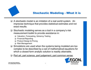
Stochastic Modeling - What it is
 A stochastic model is an imitation of a real world system. An
imprecise technique that provides statistical estimates and not
exact results.
 Stochastic modeling serves as a tool in a company’s risk
measurement toolkit to provide assistance in:
 Valuation, Forecasting, Solvency Testing
 Financial Reporting
 Product Design & Pricing
 Risk Management
 Simulations are used when the systems being modeled are too
complex to be described by a set of mathematical equations for
which a closed form analytic solution is readily attainable.
 Part art, part science, part judgement, part common sense.
SoA Stochastic Modeling
for Leading Edge Actuaries 5
Stochastic Modeling - And What it isn’t
 Not a magical solution! One needs to:
 Perform reality checks
 Understand strengths & limitations of the model
 Results are not always intuitively obvious!
 Often requires a different way of looking at problems, issues,
results, and potential solutions.
 Greater exposure to model risk and operational risks.
SoA Stochastic Modeling
for Leading Edge Actuaries 6
Advantages of Stochastic Modeling
 Systems with long time frames can be studied in compressed time.
 Able to assist in decision making and to quantify future outcomes
arising from different actions/strategies before implementation.
 Can attempt to better understand properties of real world systems
such as policyholder behavior.
 Quantification of the benefit from risk diversification.
 Coherent articulation of risk profiles.
 Potential reserve and regulatory capital relief.
SoA Stochastic Modeling
for Leading Edge Actuaries 7
Limitations of Stochastic Modeling
 Requires a considerable investment of time and expertise.
 Technically challenging, computationally demanding.
 Reliance on a few “good” people!
 For any given set of inputs, each scenario gives only a estimate.
 May create a false sense of confidence - a false sense of
precision let alone a false sense of accuracy.
 Relies heavily on data inputs and the identification of variable
interactions.
 It is not possible to include all future events in a model.
 Results may be difficult to interpret.
 Effective communication of results may be even more difficult.
 Garbage in, Garbage out!
SoA Stochastic Modeling
for Leading Edge Actuaries 8
Stochastic modeling is Preferred over
Deterministic Modeling When:
 Product or Line of Business has a “cliff” or “tail” risk profile.
 Risks are dependent and/or there is path dependence.
 When dealing with skewed and/or discontinuous distributions/cost
functions.
 Outcomes are sensitive to initial conditions.
 There is significant volatility in the underlying variables.
 Volatility or skewness of underlying variables is likely to change
over time.
 There are real economic incentives, such as reserve or capital
relief, to perform stochastic modeling.
SoA Stochastic Modeling
for Leading Edge Actuaries 9
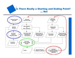
Is There Really a Starting and Ending Point?
… No!
Output
Historical
Economic Data
Historical
Policyholder
Data
Random Number
Generator
Economic
Scenario
Generator (ESG)
Stochastic ESG
Parameters &
Assumptions
Policyholder
Input Data
Economic
Scenarios
Data Validation
&
ESG Calibration
Random
Numbers
Stochastic
Asset / Liability
Models
Liability Data
Validation
Deterministic &
Stochastic Liability
Assumptions
Deterministic &
Stochastic Asset
Assumptions
Result Tabulation,
Validation, & Review
Reported
Financial Results,
Risk Management
Measures
SoA Stochastic Modeling
for Leading Edge Actuaries 10
Where does one Start? Key Steps Are ...
 Identify the key issues, objectives and potential roadblocks
before considering ways of solving the problem.
 Articulate the process / model in general terms before
proceeding to the specific.
 Develop the model: assumptions, input parameters, data,
output.
 Fit the model: gather and analyze data, estimate input
parameters
 Implement the model.
 Analyze and test sensitivity of the model results & loop back.
 Communicate the results.
SoA Stochastic Modeling
for Leading Edge Actuaries 11
Points to Keep in Mind!
 Stochastic modeling is an evolutionary / revolutionary concept.
 There must be a constant feedback loop.
 Learn to “walk” before you “run”.
 Recognize that no one model fits all solutions.
 Be careful of becoming “married to the method”, rather than the
objective.
 Keep it simple, keep it practical, keep it understandable.
 Keep performing validation and reality checks throughout all
modeling steps.
 Strive towards the production of actionable information!
SoA Stochastic Modeling
for Leading Edge Actuaries 12
Conditional Tail Expectation
 Conditional Tail Expectation (CTE) is a conditional expected value
based on downside risk.
 CTE can be defined as the average of outcomes that exceed a
specified percentile.
 The CTE(Q%) is calculated as the arithmetic average of the worst
(100-Q)% results of the stochastic simulation.
 For example: CTE(75%) is the arithmetic average of the worst
25% of the results of the stochastic simulation.
 CTE is considered to be a more robust measure with greater
information content than percentiles.
 The CTE measure can also be “modified”.
SoA Stochastic Modeling
for Leading Edge Actuaries 13
Random Number Generator
 Objective:
 To produce random numbers between 0 and 1
 Issues:
 The Random Number Generator (RNG) is a foundation building block
 Critical, but often ignored/forgotten about!
 Poor RNG can compromise all post modeling sophistication
 Numerous RNGs to choose from
 Desirable Characteristics to check for:
 Robustness independent of the seed number
 Periodicity
 Fast, efficient, & effective algorithm
 Other statistical tests (an internet search will provide many)
SoA Stochastic Modeling
for Leading Edge Actuaries 14
Economic Scenario Generator
 Objective:
 To produce capital market or economic scenarios
 Components:
 Drift, Diffusion, Correlation, …
 Issues:
 Is the focus on the mean, median, or tail events?
 What metric is of concern?
 Economic vs. Statistical model, Arbitrage-Free vs. Equilibrium
 What is our calibration benchmark?
 Numerous ESGs to choose from
 Desirable Characteristics to check for:
 Integrated model (equity, interest rate, inflation, currency)
 Incorporates the principle of parsimony.
 Flexible. A component approach.
SoA Stochastic Modeling
for Leading Edge Actuaries 15
Calibration of the
Economic Scenario Generator
 Stability of the components over time
 Drift Stability versus Diffusion Stability versus Correlation Stability
 Frequency of recalibration
 Historical data period versus forecast horizon
 Selection of lead index
 Selection of starting regime if using a multiple regime model
 Foreign exchange Issues
 Data sources and Caveat Emptor
 Approaches to fitting the data
 Risk-Return relationship
 False sense of precision and subjectivity
SoA Stochastic Modeling
for Leading Edge Actuaries 16
Example: Variable Annuity GMIB Rider
 Product:
 Guaranteed Minimum Income Benefit Rider
 Objective:
 Produce Measures for Financial Reporting
 Calculate Reserve & Capital Requirements
 Nature of the Situation:
 Case #1: MV = $1.00B, GV = $1.40B (in-the-money)
 Case #2: MV = $2.75B, GV = $2.75B (at-the-money)
 Mixture of policyholders
 5% Roll-up rate per annum
 Conservative interest and mortality assumptions at time of product
pricing
SoA Stochastic Modeling
for Leading Edge Actuaries 17
Economic Scenario Generation
 Economic Scenario Generator:
 Equity returns modeled using RSLN2 model
 Fixed Income returns modeled using Cox-Ingersol-Ross model
 Correlated Equity & Fixed Income Returns
 Calibration Method:
 Maximum Likelihood Estimation
 Calibration Issues:
 Data is limited and often inconsistent/incorrect.
 Insufficient effort is often given to data validation.
 Requires complex methods
 Historical data period versus forecast horizon
 Frequency of recalibration
 Simulation:
 1000 scenarios, monthly frequency,
30 year projection horizon
SoA Stochastic Modeling
for Leading Edge Actuaries 18
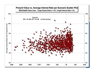
Present Value vs. Average Interest Rate per Scenario Scatter Plot
Stochastic Base Case: Target Equity Return = 8%, Target Interest Rate = 6%
2%
4%
6%
8%
10%
12%
-$300 -$250 -$200 -$150 -$100 -$50 $0 $50 $100
AverageInterestRateoverProjectionHorizon
2%
4%
6%
8%
10%
12%
Case #1:
MV = $1.0B, GV = $1.4B (in-the-money)
SoA Stochastic Modeling
for Leading Edge Actuaries 19
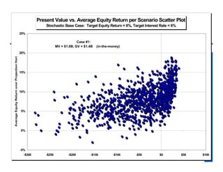
Present Value vs. Average Equity Return per Scenario Scatter Plot
Stochastic Base Case: Target Equity Return = 8%, Target Interest Rate = 6%
-5%
0%
5%
10%
15%
20%
25%
-$300 -$250 -$200 -$150 -$100 -$50 $0 $50 $100
AverageEquityReturnoverProjectionHorizon
Case #1:
MV = $1.0B, GV = $1.4B (in-the-money)
SoA Stochastic Modeling
for Leading Edge Actuaries 20
CTE Percentile
100% -$481.9 -$481.9
95% -$247.9 -$164.0
90% -$187.6 -$97.5
85% -$151.4 -$64.2
80% -$126.7 -$42.2
75% -$107.3 -$18.3
70% -$90.6 $1.7
65% -$76.4 $15.1
60% -$64.3 $24.3
55% -$54.0 $32.8
50% -$45.0 $38.0
45% -$37.2 $44.6
40% -$30.1 $50.1
35% -$23.8 $54.0
30% -$18.1 $56.9
25% -$13.0 $60.1
20% -$8.3 $65.2
15% -$3.8 $70.8
10% $0.5 $76.2
5% $4.8 $88.3
0% $9.7 $137.6
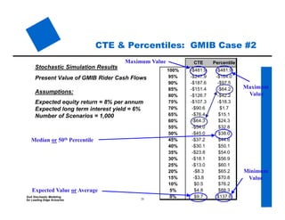
CTE & Percentiles: GMIB Case #2
Stochastic Simulation Results
Present Value of GMIB Rider Cash Flows
Assumptions:
Expected equity return = 8% per annum
Expected long term interest yield = 6%
Number of Scenarios = 1,000
Expected Value or Average
Median or 50th Percentile
Maximum Value
Maximum
Value
Minimum
Value
SoA Stochastic Modeling
for Leading Edge Actuaries 21
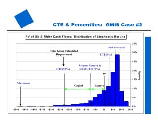
PV of GMIB Rider Cash Flow s: Distribution of Stochastic Results
0%
5%
10%
15%
20%
25%
30%
35%
-$500 -$450 -$400 -$350 -$300 -$250 -$200 -$150 -$100 -$50 $0 $50 $100 $150
Probability
CTE(0%)
50th Percentile
Assume Reserve is
set at CTE(70%)CTE(95%)
Capital
$0
Reserve
Total Gross Calculated
Requirement
Maximum
CTE & Percentiles: GMIB Case #2
SoA Stochastic Modeling
for Leading Edge Actuaries 22
Sensitivity/Stress Testing
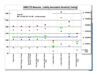
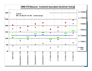
 Quantifies the impact of an immediate change in an
assumption or variable.
 Useful for validation of the model with respect to individual
assumptions
 Also a check on the modeled variable interactions
 Allows one to identify and thereby direct more effort on key
assumptions or variables.
SoA Stochastic Modeling
for Leading Edge Actuaries 23
GMIB CTE Measures: Liability Assumption Sensitivity Testing
$0
$50
$100
$150
$200
$250
$300 BaseCase
RiderCharge-10bps
CurrentPricing
Spread-10bps
Pre-AnnMortDecr
10%
Post-AnnMortDecr
10%
LapseRatex2
LapseRatex0.5
AnnuitizationRatex2
AnnuitizaionRate
x0.5
CTE(95%)
CTE(90%)
CTE(80%)
CTE(70%)
CTE(60%)
CTE(0%)
Base
Case
Case #1:
MV = $1.0B, GV = $1.4B (in-the-money)
SoA Stochastic Modeling
for Leading Edge Actuaries 24
GMIB CTE Measures: Investment Assumption Sensitivity Testing
$0
$50
$100
$150
$200
$250
$300 BaseCase
EquityReturn=10%
EquityReturn=9%
EquityReturn=7%
EquityReturn=6%
LTYield=8%
LTYield=7%
LTYield=5%
LTYield=4%
CTE(95%)
CTE(90%)
CTE(80%)
CTE(70%)
CTE(60%)
CTE(0%)
Base
Case
Case #1:
MV = $1.0B, GV = $1.4B (in-the-money)
SoA Stochastic Modeling
for Leading Edge Actuaries 25
Recommended Practices:
 Keep focused on the business objectives.
 No one model fits all. Best to understand fundamentals.
 Cultivate “best practices”.
 Keep it simple and practical.
 Focus on accuracy first, precision second.
 Add complexity on a cost/benefit basis.
 Don’t ignore data validation and model validation procedures.
 Continually perform reality checks.
 Constantly loop back through the process.
SoA Stochastic Modeling
for Leading Edge Actuaries 26
Other Issues to Wrestle With:
 Some model set-ups generate more volatility in results than
others. How do we choose between them?
 How do we perform calibration and parameter estimation?
 How do we capture the correlations between markets.
 How many scenarios do we use?
 How do we model policyholder behaviour?
 How do we incorporate hedging in the model?
SoA Stochastic Modeling
for Leading Edge Actuaries 27
Finally, Where Are We Going … ???
 Will stochastic modeling change the way the insurance industry
conducts business?
 What will be the impact of the recent acceptance/application of
stochastic modeling within the next 1, 5, 10+ years?
 How will stochastic modeling alter/impact pricing, product
development, and valuation / risk management practices &
procedures?
 Even closer to home, how will stochastic modeling impact the
educational experience and skill requirements of current and
future actuaries?
SoA Stochastic Modeling
for Leading Edge Actuaries 28
Wrap-Up
Questions & Answers!

Practical Aspects of Stochastic Modeling.pptx

  • 1.
    SoA Stochastic Modeling forLeading Edge Actuaries 1 Stochastic Modeling for Leading Edge Actuaries Overview of the Practical Aspects of Stochastic Modeling Ron Harasym MBA, CFA, FSA, FCIA Vice-President & Chief Risk Officer
  • 2.
    SoA Stochastic Modeling forLeading Edge Actuaries 2 Outline of Presentation  Stochastic Modeling Defined.  What Stochastic Modeling is and isn’t.  Advantages and Limitations of Stochastic Modeling.  When Stochastic Modeling is Preferred.  Key steps in Stochastic Modeling  Conditional Tail Expectation & Examples  Recommended Practices  Final Thoughts
  • 3.
    SoA Stochastic Modeling forLeading Edge Actuaries 3 Stochastic Modeling - Definition  Stochastic [Greek stokhastikos: from stokhasts, diviner, from stokhazesthai, to guess at, from stokhos, aim, goal.]  A stochastic model by definition has at least one random variable and deals explicitly with time-variable interaction.  A stochastic simulation uses a statistical sampling of multiple replicates, repeated simulations, of the same model.  Such simulations are also sometimes referred to as Monte Carlo simulations because of their use of random variables.
  • 4.
    SoA Stochastic Modeling forLeading Edge Actuaries 4 Stochastic Modeling - What it is  A stochastic model is an imitation of a real world system. An imprecise technique that provides statistical estimates and not exact results.  Stochastic modeling serves as a tool in a company’s risk measurement toolkit to provide assistance in:  Valuation, Forecasting, Solvency Testing  Financial Reporting  Product Design & Pricing  Risk Management  Simulations are used when the systems being modeled are too complex to be described by a set of mathematical equations for which a closed form analytic solution is readily attainable.  Part art, part science, part judgement, part common sense.
  • 5.
    SoA Stochastic Modeling forLeading Edge Actuaries 5 Stochastic Modeling - And What it isn’t  Not a magical solution! One needs to:  Perform reality checks  Understand strengths & limitations of the model  Results are not always intuitively obvious!  Often requires a different way of looking at problems, issues, results, and potential solutions.  Greater exposure to model risk and operational risks.
  • 6.
    SoA Stochastic Modeling forLeading Edge Actuaries 6 Advantages of Stochastic Modeling  Systems with long time frames can be studied in compressed time.  Able to assist in decision making and to quantify future outcomes arising from different actions/strategies before implementation.  Can attempt to better understand properties of real world systems such as policyholder behavior.  Quantification of the benefit from risk diversification.  Coherent articulation of risk profiles.  Potential reserve and regulatory capital relief.
  • 7.
    SoA Stochastic Modeling forLeading Edge Actuaries 7 Limitations of Stochastic Modeling  Requires a considerable investment of time and expertise.  Technically challenging, computationally demanding.  Reliance on a few “good” people!  For any given set of inputs, each scenario gives only a estimate.  May create a false sense of confidence - a false sense of precision let alone a false sense of accuracy.  Relies heavily on data inputs and the identification of variable interactions.  It is not possible to include all future events in a model.  Results may be difficult to interpret.  Effective communication of results may be even more difficult.  Garbage in, Garbage out!
  • 8.
    SoA Stochastic Modeling forLeading Edge Actuaries 8 Stochastic modeling is Preferred over Deterministic Modeling When:  Product or Line of Business has a “cliff” or “tail” risk profile.  Risks are dependent and/or there is path dependence.  When dealing with skewed and/or discontinuous distributions/cost functions.  Outcomes are sensitive to initial conditions.  There is significant volatility in the underlying variables.  Volatility or skewness of underlying variables is likely to change over time.  There are real economic incentives, such as reserve or capital relief, to perform stochastic modeling.
  • 9.
    SoA Stochastic Modeling forLeading Edge Actuaries 9 Is There Really a Starting and Ending Point? … No! Output Historical Economic Data Historical Policyholder Data Random Number Generator Economic Scenario Generator (ESG) Stochastic ESG Parameters & Assumptions Policyholder Input Data Economic Scenarios Data Validation & ESG Calibration Random Numbers Stochastic Asset / Liability Models Liability Data Validation Deterministic & Stochastic Liability Assumptions Deterministic & Stochastic Asset Assumptions Result Tabulation, Validation, & Review Reported Financial Results, Risk Management Measures
  • 10.
    SoA Stochastic Modeling forLeading Edge Actuaries 10 Where does one Start? Key Steps Are ...  Identify the key issues, objectives and potential roadblocks before considering ways of solving the problem.  Articulate the process / model in general terms before proceeding to the specific.  Develop the model: assumptions, input parameters, data, output.  Fit the model: gather and analyze data, estimate input parameters  Implement the model.  Analyze and test sensitivity of the model results & loop back.  Communicate the results.
  • 11.
    SoA Stochastic Modeling forLeading Edge Actuaries 11 Points to Keep in Mind!  Stochastic modeling is an evolutionary / revolutionary concept.  There must be a constant feedback loop.  Learn to “walk” before you “run”.  Recognize that no one model fits all solutions.  Be careful of becoming “married to the method”, rather than the objective.  Keep it simple, keep it practical, keep it understandable.  Keep performing validation and reality checks throughout all modeling steps.  Strive towards the production of actionable information!
  • 12.
    SoA Stochastic Modeling forLeading Edge Actuaries 12 Conditional Tail Expectation  Conditional Tail Expectation (CTE) is a conditional expected value based on downside risk.  CTE can be defined as the average of outcomes that exceed a specified percentile.  The CTE(Q%) is calculated as the arithmetic average of the worst (100-Q)% results of the stochastic simulation.  For example: CTE(75%) is the arithmetic average of the worst 25% of the results of the stochastic simulation.  CTE is considered to be a more robust measure with greater information content than percentiles.  The CTE measure can also be “modified”.
  • 13.
    SoA Stochastic Modeling forLeading Edge Actuaries 13 Random Number Generator  Objective:  To produce random numbers between 0 and 1  Issues:  The Random Number Generator (RNG) is a foundation building block  Critical, but often ignored/forgotten about!  Poor RNG can compromise all post modeling sophistication  Numerous RNGs to choose from  Desirable Characteristics to check for:  Robustness independent of the seed number  Periodicity  Fast, efficient, & effective algorithm  Other statistical tests (an internet search will provide many)
  • 14.
    SoA Stochastic Modeling forLeading Edge Actuaries 14 Economic Scenario Generator  Objective:  To produce capital market or economic scenarios  Components:  Drift, Diffusion, Correlation, …  Issues:  Is the focus on the mean, median, or tail events?  What metric is of concern?  Economic vs. Statistical model, Arbitrage-Free vs. Equilibrium  What is our calibration benchmark?  Numerous ESGs to choose from  Desirable Characteristics to check for:  Integrated model (equity, interest rate, inflation, currency)  Incorporates the principle of parsimony.  Flexible. A component approach.
  • 15.
    SoA Stochastic Modeling forLeading Edge Actuaries 15 Calibration of the Economic Scenario Generator  Stability of the components over time  Drift Stability versus Diffusion Stability versus Correlation Stability  Frequency of recalibration  Historical data period versus forecast horizon  Selection of lead index  Selection of starting regime if using a multiple regime model  Foreign exchange Issues  Data sources and Caveat Emptor  Approaches to fitting the data  Risk-Return relationship  False sense of precision and subjectivity
  • 16.
    SoA Stochastic Modeling forLeading Edge Actuaries 16 Example: Variable Annuity GMIB Rider  Product:  Guaranteed Minimum Income Benefit Rider  Objective:  Produce Measures for Financial Reporting  Calculate Reserve & Capital Requirements  Nature of the Situation:  Case #1: MV = $1.00B, GV = $1.40B (in-the-money)  Case #2: MV = $2.75B, GV = $2.75B (at-the-money)  Mixture of policyholders  5% Roll-up rate per annum  Conservative interest and mortality assumptions at time of product pricing
  • 17.
    SoA Stochastic Modeling forLeading Edge Actuaries 17 Economic Scenario Generation  Economic Scenario Generator:  Equity returns modeled using RSLN2 model  Fixed Income returns modeled using Cox-Ingersol-Ross model  Correlated Equity & Fixed Income Returns  Calibration Method:  Maximum Likelihood Estimation  Calibration Issues:  Data is limited and often inconsistent/incorrect.  Insufficient effort is often given to data validation.  Requires complex methods  Historical data period versus forecast horizon  Frequency of recalibration  Simulation:  1000 scenarios, monthly frequency, 30 year projection horizon
  • 18.
    SoA Stochastic Modeling forLeading Edge Actuaries 18 Present Value vs. Average Interest Rate per Scenario Scatter Plot Stochastic Base Case: Target Equity Return = 8%, Target Interest Rate = 6% 2% 4% 6% 8% 10% 12% -$300 -$250 -$200 -$150 -$100 -$50 $0 $50 $100 AverageInterestRateoverProjectionHorizon 2% 4% 6% 8% 10% 12% Case #1: MV = $1.0B, GV = $1.4B (in-the-money)
  • 19.
    SoA Stochastic Modeling forLeading Edge Actuaries 19 Present Value vs. Average Equity Return per Scenario Scatter Plot Stochastic Base Case: Target Equity Return = 8%, Target Interest Rate = 6% -5% 0% 5% 10% 15% 20% 25% -$300 -$250 -$200 -$150 -$100 -$50 $0 $50 $100 AverageEquityReturnoverProjectionHorizon Case #1: MV = $1.0B, GV = $1.4B (in-the-money)
  • 20.
    SoA Stochastic Modeling forLeading Edge Actuaries 20 CTE Percentile 100% -$481.9 -$481.9 95% -$247.9 -$164.0 90% -$187.6 -$97.5 85% -$151.4 -$64.2 80% -$126.7 -$42.2 75% -$107.3 -$18.3 70% -$90.6 $1.7 65% -$76.4 $15.1 60% -$64.3 $24.3 55% -$54.0 $32.8 50% -$45.0 $38.0 45% -$37.2 $44.6 40% -$30.1 $50.1 35% -$23.8 $54.0 30% -$18.1 $56.9 25% -$13.0 $60.1 20% -$8.3 $65.2 15% -$3.8 $70.8 10% $0.5 $76.2 5% $4.8 $88.3 0% $9.7 $137.6 CTE & Percentiles: GMIB Case #2 Stochastic Simulation Results Present Value of GMIB Rider Cash Flows Assumptions: Expected equity return = 8% per annum Expected long term interest yield = 6% Number of Scenarios = 1,000 Expected Value or Average Median or 50th Percentile Maximum Value Maximum Value Minimum Value
  • 21.
    SoA Stochastic Modeling forLeading Edge Actuaries 21 PV of GMIB Rider Cash Flow s: Distribution of Stochastic Results 0% 5% 10% 15% 20% 25% 30% 35% -$500 -$450 -$400 -$350 -$300 -$250 -$200 -$150 -$100 -$50 $0 $50 $100 $150 Probability CTE(0%) 50th Percentile Assume Reserve is set at CTE(70%)CTE(95%) Capital $0 Reserve Total Gross Calculated Requirement Maximum CTE & Percentiles: GMIB Case #2
  • 22.
    SoA Stochastic Modeling forLeading Edge Actuaries 22 Sensitivity/Stress Testing  Quantifies the impact of an immediate change in an assumption or variable.  Useful for validation of the model with respect to individual assumptions  Also a check on the modeled variable interactions  Allows one to identify and thereby direct more effort on key assumptions or variables.
  • 23.
    SoA Stochastic Modeling forLeading Edge Actuaries 23 GMIB CTE Measures: Liability Assumption Sensitivity Testing $0 $50 $100 $150 $200 $250 $300 BaseCase RiderCharge-10bps CurrentPricing Spread-10bps Pre-AnnMortDecr 10% Post-AnnMortDecr 10% LapseRatex2 LapseRatex0.5 AnnuitizationRatex2 AnnuitizaionRate x0.5 CTE(95%) CTE(90%) CTE(80%) CTE(70%) CTE(60%) CTE(0%) Base Case Case #1: MV = $1.0B, GV = $1.4B (in-the-money)
  • 24.
    SoA Stochastic Modeling forLeading Edge Actuaries 24 GMIB CTE Measures: Investment Assumption Sensitivity Testing $0 $50 $100 $150 $200 $250 $300 BaseCase EquityReturn=10% EquityReturn=9% EquityReturn=7% EquityReturn=6% LTYield=8% LTYield=7% LTYield=5% LTYield=4% CTE(95%) CTE(90%) CTE(80%) CTE(70%) CTE(60%) CTE(0%) Base Case Case #1: MV = $1.0B, GV = $1.4B (in-the-money)
  • 25.
    SoA Stochastic Modeling forLeading Edge Actuaries 25 Recommended Practices:  Keep focused on the business objectives.  No one model fits all. Best to understand fundamentals.  Cultivate “best practices”.  Keep it simple and practical.  Focus on accuracy first, precision second.  Add complexity on a cost/benefit basis.  Don’t ignore data validation and model validation procedures.  Continually perform reality checks.  Constantly loop back through the process.
  • 26.
    SoA Stochastic Modeling forLeading Edge Actuaries 26 Other Issues to Wrestle With:  Some model set-ups generate more volatility in results than others. How do we choose between them?  How do we perform calibration and parameter estimation?  How do we capture the correlations between markets.  How many scenarios do we use?  How do we model policyholder behaviour?  How do we incorporate hedging in the model?
  • 27.
    SoA Stochastic Modeling forLeading Edge Actuaries 27 Finally, Where Are We Going … ???  Will stochastic modeling change the way the insurance industry conducts business?  What will be the impact of the recent acceptance/application of stochastic modeling within the next 1, 5, 10+ years?  How will stochastic modeling alter/impact pricing, product development, and valuation / risk management practices & procedures?  Even closer to home, how will stochastic modeling impact the educational experience and skill requirements of current and future actuaries?
  • 28.
    SoA Stochastic Modeling forLeading Edge Actuaries 28 Wrap-Up Questions & Answers!