Download as PDF, PPTX

![Importance Sampling
10.1 Variational Inference 8
IntegralBasic idea:
Transform the integral
into an expectation over a
simple, known
distribution
p(z) f(z)
z
q(z)
Conditions:
• q(z) > 0 when f(z)p(z) ≠ 0
• Easy to sample from q(z)
E[f] =
Z
f(z)p(z)dz
E[f] =
Z
f(z)p(z)
q(z)
q(z)
dz
Notice: x is abbreviated in formula
E[f] =
Z
f(z)
p(z)
q(z)
q(z)dz
w(s)
=
p(z(s)
)
q(z(s))
z(s)
⇠ q(z)
E[f] =
1
S
X
s
w(s)
f(z(s)
)
Proposal
Importance
weight
Monte Carlo](https://image.slidesharecdn.com/prmlreadingchapter10approximateinference-151228152004/75/Approximate-Inference-Chapter-10-PRML-Reading-8-2048.jpg)
![Importance Sampling
10.1 Variational Inference 9
p(z) f(z)
z
q(z)
Properties:
• Unbiased estimate of the expectation
• No independent samples from posterior
distribution
• Many draws from proposal needed,
especially in high dimensions
E[f] =
1
S
X
s
w(s)
f(z(s)
)
w(s)
=
p(z(s)
)
q(z(s))
z(s)
⇠ q(z)
Stochastic
Approximation
Chapter 11](https://image.slidesharecdn.com/prmlreadingchapter10approximateinference-151228152004/75/Approximate-Inference-Chapter-10-PRML-Reading-9-2048.jpg)
![Importance Sampling
10.1 Variational Inference 10
p(z) f(z)
z
q(z)
Take inspiration from importance sampling, but instead:
• Obtain a deterministic algorithm
• Scaled up to high-dimensional and large data problems
• Easy convergence assessment
E[f] =
1
S
X
s
w(s)
f(z(s)
)
w(s)
=
p(z(s)
)
q(z(s))
z(s)
⇠ q(z)
Variational
Inference](https://image.slidesharecdn.com/prmlreadingchapter10approximateinference-151228152004/75/Approximate-Inference-Chapter-10-PRML-Reading-10-2048.jpg)
![Variational Calculus
10.1 Variational Inference 12
Functions:
• Variables as input, output is a value
• Full and partial derivatives df/dx
• Ex. Maximize likelihood p(x|µ) w.r.t.
parameters µ
Both types of derivatives are
exploited in variational inference
Functionals:
• Functions as input, output is a value
• Functional derivatives ∂f/∂x
• Ex. Maximize the entropy H[p(x)] w.r.t.
p(x)
Variational method derives from the
Calculus of Variations](https://image.slidesharecdn.com/prmlreadingchapter10approximateinference-151228152004/75/Approximate-Inference-Chapter-10-PRML-Reading-12-2048.jpg)
![From IS to Variational Inference
10.1 Variational Inference 13
Integral
Importance weight
Jensen’s inequality
ln p(X) = ln
Z
p(X|Z)p(Z)dZ
ln p(X) = ln
Z
p(X|Z)
p(Z)
q(Z)
q(Z)dZ
ln
Z
p(x)g(x)dx
Z
p(x) ln g(x)dx
ln p(X)
Z
q(Z) ln (p(X|Z)
p(Z)
q(Z)
)dZ
Variational
(evidence) lower
bound
=
Z
q(Z) ln p(X|Z)dZ
Z
q(Z) ln
q(Z)
p(Z)
dZ
Eq(Z)[ln p(X|Z)] KL[q(Z)||p(Z)]=](https://image.slidesharecdn.com/prmlreadingchapter10approximateinference-151228152004/75/Approximate-Inference-Chapter-10-PRML-Reading-13-2048.jpg)
![Variational Lower Bound
10.1 Variational Inference 14
F(X, q) =
Reconstruction PenaltyApprox. Posterior
• Penalty: Ensures the explanation of the data q(Z) doesn’t deviate too far from
your beliefs p(Z).
• Reconstruction cost: The expected log-likelihood measure how well samples
from q(Z) are able to explain the data X.
• Approximate posterior distribution q(Z): Best match to true posterior p(Z|X),
one of the unknown inferential quantities of interest to us.
Interpreting the bound:
Eq(Z)[ln p(X|Z)] KL[q(Z)||p(Z)]](https://image.slidesharecdn.com/prmlreadingchapter10approximateinference-151228152004/75/Approximate-Inference-Chapter-10-PRML-Reading-14-2048.jpg)
![How low the VLB (ELB)?
10.1 Variational Inference 15
• Variational parameters: Parameters of q(Z) (Ex. if a Gaussian, they’re mean
and variance).
• Integration switched to optimization: optimize q(Z) directly (my thought:
actually it is q(Z|X) ) to minimize
Some comments on q:
ln p(X) F(X, q) =
Z
q(Z) ln p(X)dZ F(X, q)
=
Z
q(Z) ln p(X)dZ
Z
q(Z) ln p(X|Z)dZ +
Z
q(Z) ln
q(Z)
p(Z)
dZ
=
Z
q(Z) ln
p(X)q(Z)
p(X|Z)p(Z)
dZ =
Z
q(Z) ln
q(Z)
p(Z|X)
dZ
= KL[q(Z)||p(Z|X)]
KL[q(Z)||p(Z|X)]](https://image.slidesharecdn.com/prmlreadingchapter10approximateinference-151228152004/75/Approximate-Inference-Chapter-10-PRML-Reading-15-2048.jpg)
![Factorized distributions (II)
10.1 Variational Inference 19
L(q) =
Z
q(Z) ln
⇢
p(X, Z)
q(Z)
dZ
=
Z
q(Z) {ln p(X, Z) ln q(Z)} dZ
=
Z Y
i
qi(Zi)
! (
ln p(X, Z)
X
i
ln qi(Zi)
)
dZ
=
Z Y
i
qi
!
[ln p(X, Z)] dZ
Z Y
i
qi
!
X
i
ln qi
!
dZ
qi](https://image.slidesharecdn.com/prmlreadingchapter10approximateinference-151228152004/75/Approximate-Inference-Chapter-10-PRML-Reading-19-2048.jpg)
![Factorized distributions (III)
10.1 Variational Inference 20
L(q) =
Z Y
i
qi
!
[ln p(X, Z)] dZ
Z Y
i
qi
!
X
i
ln qi
!
dZ
=
Z
qj
8
<
:
Z
ln p(X, Z)
Y
i6=j
qidZi
9
=
;
dZj
Z Y
i
qi
! 8
<
:
ln qj +
X
i6=j
ln qi
9
=
;
dZ
=
Z
qj
8
<
:
Z
ln p(X, Z)
Y
i6=j
qidZi
9
=
;
dZj
Z Y
i
qi
!
ln qjdZ
Z
0
@
Y
i6=j
qi
1
A
0
@
X
i6=j
ln qi
1
A
✓Z
qjdZj
◆
dZi6=j
=
Z
qj (ln ˜p(X, Zj) const) dZj
Z
qj ln qjdZj
Z
0
@
Y
i6=j
qi
1
A
0
@
X
i6=j
ln qi
1
A dZi6=j
• Consider with function qj(Zj)
= 1](https://image.slidesharecdn.com/prmlreadingchapter10approximateinference-151228152004/75/Approximate-Inference-Chapter-10-PRML-Reading-20-2048.jpg)
![Factorized distributions (IV)
10.1 Variational Inference 21
L(q) =
Z
qj ln ˜p(X, Zj)dZj
Z
qj ln qjdZj + const
negative KL divergence
where
˜p(X, Zj) = Ei6=j[ln p(X, Z)] + const
Ei6=j[ln p(X, Z)] =
Z
ln p(X, Z)
Y
i6=j
qidZi
and
• Maximize by keeping fixed
• This is same as minimizing KL divergence between
and
L(q) {qi6=j}
˜p(X, Zj)
qj(Zj)
(10.6)
(10.7)
(10.8)](https://image.slidesharecdn.com/prmlreadingchapter10approximateinference-151228152004/75/Approximate-Inference-Chapter-10-PRML-Reading-21-2048.jpg)
![Optimal Solution
10.1 Variational Inference 22
(1) Initialize all qj appropriately.
ln q⇤
j (Zj) = Ei6=j[ln p(X, Z)] + const
q⇤
j (Zj) =
exp(Ei6=j[ln p(X, Z)])
R
exp(Ei6=j[ln p(X, Z)])dZj
or
(2) Run below code until convergence.
• foreach qi
• Fixed all qj ≠qi and find optimal qi
• Update qi
(10.9)Today’s
memo
Next slides are
detailed examples](https://image.slidesharecdn.com/prmlreadingchapter10approximateinference-151228152004/75/Approximate-Inference-Chapter-10-PRML-Reading-22-2048.jpg)
![10.1.2. Properties of factorized approximations
10.1 Variational Inference 23
Approximate Gaussian Distribution with factorized Gaussian
Consider,
p(z) = N(z|µ, ⇤ 1
)
µ = (µ1, µ2)T
, ⇤ =
✓
⇤11 ⇤12
⇤21 ⇤22
◆
q(z) = q1(z)q2(z)
ln q⇤
1(z1) = Ez2
[ln p(z)] + const
ln q⇤
1(z1) = Ez2 [
1
2
(z1 µ1)2
⇤11 (z1 µ1)⇤12(z2 µ2)] + const
where z = (z1, z2),
Approximate using
Optimal solution from (10.9)
consider only the terms have z1](https://image.slidesharecdn.com/prmlreadingchapter10approximateinference-151228152004/75/Approximate-Inference-Chapter-10-PRML-Reading-23-2048.jpg)
![10.1 Variational Inference 24
ln q⇤
1(z1) = Ez2 [
1
2
(z1 µ1)2
⇤11 (z1 µ1)⇤12(z2 µ2)] + const
=
Z
q2(z2)
⇢
1
2
(z1 µ1)2
⇤11 (z1 µ1)⇤12(z2 µ2) dz2 + const
=
1
2
(z1 µ1)2
⇤11 z1⇤12(Ez2 [z2] µ2) + const
q⇤
1(z1) = N(z1|m1, ⇤ 1
11 )
m1 = µ1 ⇤ 1
11 ⇤12(Ez2
[z2] µ2)
quadratic form of z1
Then, we have
(10.11)
10.1.2. Properties of factorized approximations](https://image.slidesharecdn.com/prmlreadingchapter10approximateinference-151228152004/75/Approximate-Inference-Chapter-10-PRML-Reading-24-2048.jpg)
![10.1 Variational Inference 25
q⇤
1(z1) = N(z1|m1, ⇤ 1
11 ) m1 = µ1 ⇤ 1
11 ⇤12(Ez2
[z2] µ2)
m2 = µ2 ⇤ 1
22 ⇤21(Ez1
[z1] µ1)q⇤
2(z2) = N(z2|m2, ⇤ 1
22 )
q(z) = q1(z)q2(z)Optimal solution of (10.12)-(10.15)
Mutual dependency:
• depends on (calculated by )q⇤
1(z1) q⇤
2(z2)
Ez1
[z1]
Ez2
[z2]
• depends on (calculated by )q⇤
1(z1)q⇤
2(z2)
Update alternately until convergence
10.1.2. Properties of factorized approximations](https://image.slidesharecdn.com/prmlreadingchapter10approximateinference-151228152004/75/Approximate-Inference-Chapter-10-PRML-Reading-25-2048.jpg)
![10.1 Variational Inference 26
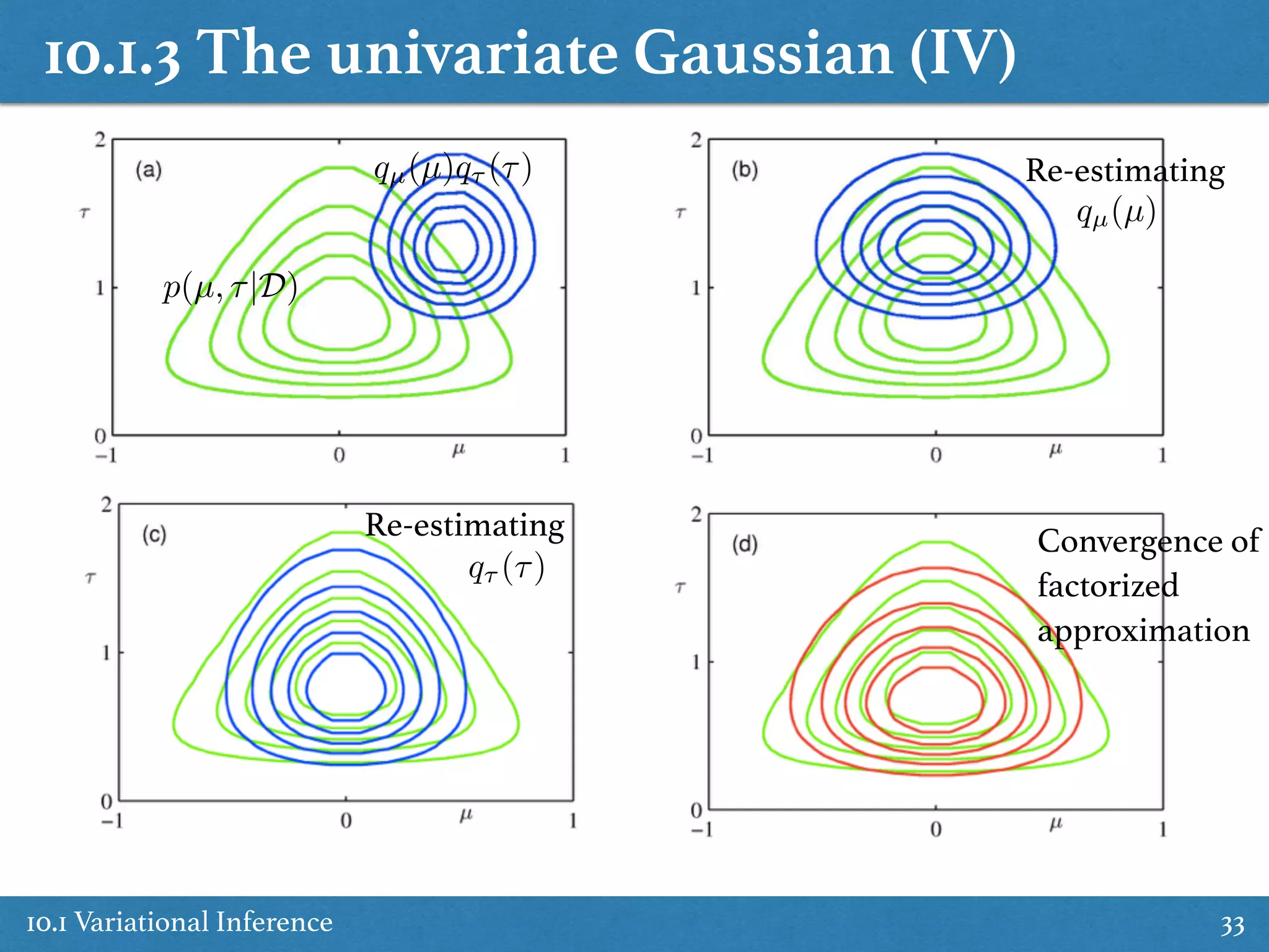
Fig 10.2 The green contours corresponding to 1, 2
and 3 standard deviations for a correlated
Gaussian distribution p(z) over two variables z1
and z2 . The red contours represent the
corresponding levels for an approximating
distribution q(z) over the same variables given by
the product of two independent univariate
Gaussian
Minimize KL(q||p) Minimize KL(p||q)
• The mean is captured correctly, but the variance is underestimated in the
orthogonal direction
• Optimal solution
(that is the corresponding marginal distribution of p(Z) )
• Considering reverse KL divergence KL(p||q) =
Z
p(Z)[
MX
i=1
ln qi(Zi)]dZ + const
10.1.2. Properties of factorized approximations
(10.17)](https://image.slidesharecdn.com/prmlreadingchapter10approximateinference-151228152004/75/Approximate-Inference-Chapter-10-PRML-Reading-26-2048.jpg)
![10.1 Variational Inference 27
Minimize KL(q||p)
Minimize KL(p||q)
Reverse KL divergence
KL(p||q) =
Z
p(Z)[
MX
i=1
ln qi(Zi)]dZ + const
10.1.2. Properties of factorized approximations
KL(q||p) =
Z
q(Z) ln
⇢
p(Z)
q(Z)
• If near zero then tends to close to zerop(Z) q(Z)
• If near zero then is not
important
p(Z) q(Z)
• KL divergence is minimized by distributions that
are nonzero in regions when is nonzerop(Z)
q(Z)](https://image.slidesharecdn.com/prmlreadingchapter10approximateinference-151228152004/75/Approximate-Inference-Chapter-10-PRML-Reading-27-2048.jpg)
![10.1.3 The univariate Gaussian (II)
10.1 Variational Inference 30
ln q⇤
µ(µ) = E⌧ [ln p(D, µ, ⌧)] + const
= E⌧ [ln (p(D|µ, ⌧)p(µ|⌧)p(⌧))] + const
= E⌧ [ln p(D|µ, ⌧) + ln p(µ|⌧) + ln p(⌧)] + const
= E⌧ [ln p(D|µ, ⌧) + ln p(µ|⌧)] + const
= E⌧
"
⌧
2
NX
n=1
(xn µ)2 0⌧
2
(µ µ0)2
#
+ const
=
E⌧ [⌧]
2
" NX
n=1
(xn µ)2
+ 0(µ µ0)2
#
+ const (10.25)
quadratic form of µ
• Optimal solution (from formula 10.9)](https://image.slidesharecdn.com/prmlreadingchapter10approximateinference-151228152004/75/Approximate-Inference-Chapter-10-PRML-Reading-30-2048.jpg)
![10.1.3 The univariate Gaussian (II)
10.1 Variational Inference 31
• Optimal solution for mean
q⇤
µ(µ) = N(µ|µN , 1
N )
8
<
:
µn =
0µ0 + N ¯x
0 + N
N = ( 0 + N)E⌧ [⌧]
where
(10.26)
(10.27)
• Similar with optimal solution of q⌧ (⌧)
q⇤
⌧ (⌧) = Eµ[ln p(D|µ, ⌧) + ln p(µ|⌧) + ln p(⌧)] + const
=
⌧
2
Eµ
" NX
n=1
(xn µ)2
+ 0(µ µ0)2
#
+
N
2
ln ⌧ +
1
2
ln ⌧ + (a0 1) ln ⌧ b0⌧ + const
=
✓
a0 +
N + 1
2
1
◆
ln ⌧
✓
b0 +
1
2
Eµ[...]
◆
⌧ + const (10.28)](https://image.slidesharecdn.com/prmlreadingchapter10approximateinference-151228152004/75/Approximate-Inference-Chapter-10-PRML-Reading-31-2048.jpg)
![10.1.3 The univariate Gaussian (III)
10.1 Variational Inference 32
• Optimal solution of q⌧ (⌧)
q⇤
⌧ (⌧) / ⌧
0
@a0+
N + 1
2
1
1
A
exp
✓ ✓
b0 +
1
2
Eµ[...]
◆
⌧
◆
or
q⇤
⌧ (⌧) = Gam(⌧|aN , bN )
where
8
><
>:
aN = a0 +
N + 1
2
bN = b0 +
1
2
Eµ
hPN
n=1(xn µ)2
+ 0(µ µ0)2
i
(10.29)
(10.30)
• Using (10.26)(10.27) and (10.29)(10.30) alternately to compute posterior
by approximate variational inference
p(µ, ⌧|D)](https://image.slidesharecdn.com/prmlreadingchapter10approximateinference-151228152004/75/Approximate-Inference-Chapter-10-PRML-Reading-32-2048.jpg)
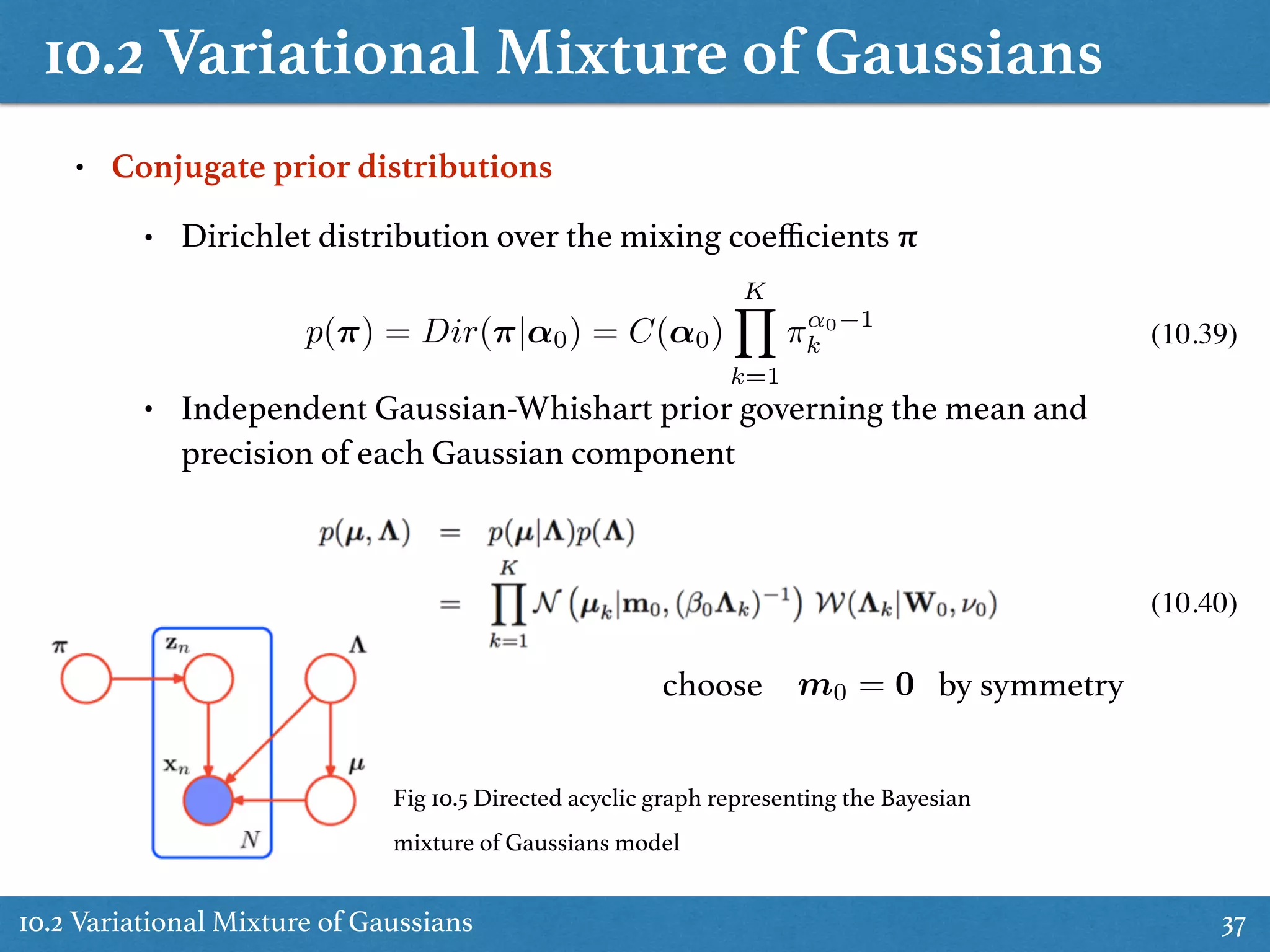
![10.2.1. Variational Distribution (I)
10.2 Variational Mixture of Gaussians 38
• Joint distribution
• Approximate
p(X, Z, ⇡, µ, ⇤) = p(X|Z, µ, ⇤)p(Z|⇡)p(⇡)p(µ|⇤)p(⇤)
q(Z, ⇡, µ, ⇤) = q(Z)q(⇡, µ, ⇤)
• Optimal solution (from formula 10.9)
ln q⇤
(Z) = E⇡,µ,⇤[ln p(X, Z, ⇡, µ, ⇤)] + const
= E⇡[ln p(Z|⇡)] + Eµ,⇤[ln p(X|Z, µ, ⇤)] + const
= E⇡
"
ln
NY
n=1
KY
k=1
⇡znk
k
!#
+ Eµ,⇤
"
ln
NY
n=1
KY
k=1
N(xn|µk, ⇤ 1
k )znk
!#
+ const
=
NX
n=1
KX
k=1
znkE⇡[ln ⇡k]
+
NX
n=1
KX
k=1
znkEµ,⇤
1
2
ln |⇤k|
D
2
ln(2⇡)
1
2
(xn µk)T
⇤k(xn µk) + const
(10.42)
(10.43)
(10.44)
D is the dimensionality of the data variable x](https://image.slidesharecdn.com/prmlreadingchapter10approximateinference-151228152004/75/Approximate-Inference-Chapter-10-PRML-Reading-38-2048.jpg)
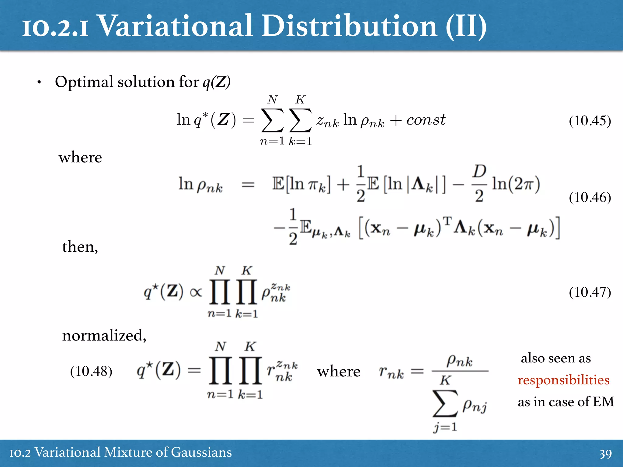
![10.2.1 Variational Distribution (III)
10.2 Variational Mixture of Gaussians 40
• Optimal solution for q(⇡, µ, ⇤)
define: (10.51)
(10.52)
(10.53)
optimal solution:
ln q⇤
(⇡, µ, ⇤) = EZ[ln p(X, Z, ⇡, µ, ⇤)] + const
= EZ[ln (p(X|Z, µ, ⇤)p(Z|⇡)p(⇡)p(µ|⇤)p(⇤))] + const
= EZ[ln p(X|Z, µ, ⇤)] + EZ[ln p(Z|⇡)] + ln p(⇡) + ln p(µ, ⇤) + const
=
NX
n=1
KX
k=1
EZ[znk] ln N(xn|µk, ⇤ 1
k ) + EZ[ln p(Z|⇡)]
+ ln p(⇡) +
KX
k=1
ln p(µk, ⇤k) + const
(10.54)](https://image.slidesharecdn.com/prmlreadingchapter10approximateinference-151228152004/75/Approximate-Inference-Chapter-10-PRML-Reading-40-2048.jpg)
![10.2.1 Variational Distribution (IV)
10.2 Variational Mixture of Gaussians 41
=
NX
n=1
KX
k=1
EZ[znk] ln N(xn|µk, ⇤ 1
k ) + EZ[ln p(Z|⇡)]
+ ln p(⇡) +
KX
k=1
ln p(µk, ⇤k) + const
ln q⇤
(⇡, µ, ⇤) ⇡
µ, ⇤
something of
+ something of
Then it could be further factorization
q(⇡, µ, ⇤) = q(⇡)
KY
k=1
q(µk, ⇤k)
q⇤
(⇡, µ, ⇤) = q⇤
(⇡)
KY
k=1
q⇤
(µk, ⇤k)
(10.54)
(10.54)
From (10.54) and (10.55) we have
ln q⇤
(⇡) = EZ[ln p(Z|⇡)] + ln p(⇡) + const
ln q⇤
(µk, ⇤k) = ln p(µk, ⇤k) +
NX
n=1
EZ[znk] ln N(xn|µk, ⇤ 1
k ) + const](https://image.slidesharecdn.com/prmlreadingchapter10approximateinference-151228152004/75/Approximate-Inference-Chapter-10-PRML-Reading-41-2048.jpg)
![10.2.1 Variational Distribution (VI)
10.2 Variational Mixture of Gaussians 42
ln q⇤
(⇡) = EZ[ln p(Z|⇡)] + ln p(⇡) + const
= EZ
"
ln
NY
n=1
KY
k=1
⇡znk
k
!#
+ ln C(↵0)
KY
k=1
⇡↵0 1
k
!
+ const
=
NX
n=1
KX
k=1
EZ[znk] ln ⇡k + (↵0 1)
KX
k=1
ln ⇡k + const
=
KX
k=1
(Nk + ↵0 1) ln ⇡k + const
= ln
KY
k=1
⇡Nk+↵0 1
k
!
+ const
q⇤
(⇡) = Dir(⇡|↵)
↵k = Nk + ↵0
is recognized as Dirichlet distributionq⇤
(⇡)
(10.56)
(10.57)
(10.58)](https://image.slidesharecdn.com/prmlreadingchapter10approximateinference-151228152004/75/Approximate-Inference-Chapter-10-PRML-Reading-42-2048.jpg)
![10.2.1 Variational Distribution (VII)
10.2 Variational Mixture of Gaussians 43
ln q⇤
(µk, ⇤k) = ln p(µk, ⇤k) +
NX
n=1
EZ[znk] ln N(xn|µk, ⇤ 1
k ) + const
We have Gaussian-Wishart distribution (exercise 10.13)
(10.59)
(10.60) - (10.63)
Analogous to the
M-step of the EM
algorithm](https://image.slidesharecdn.com/prmlreadingchapter10approximateinference-151228152004/75/Approximate-Inference-Chapter-10-PRML-Reading-43-2048.jpg)
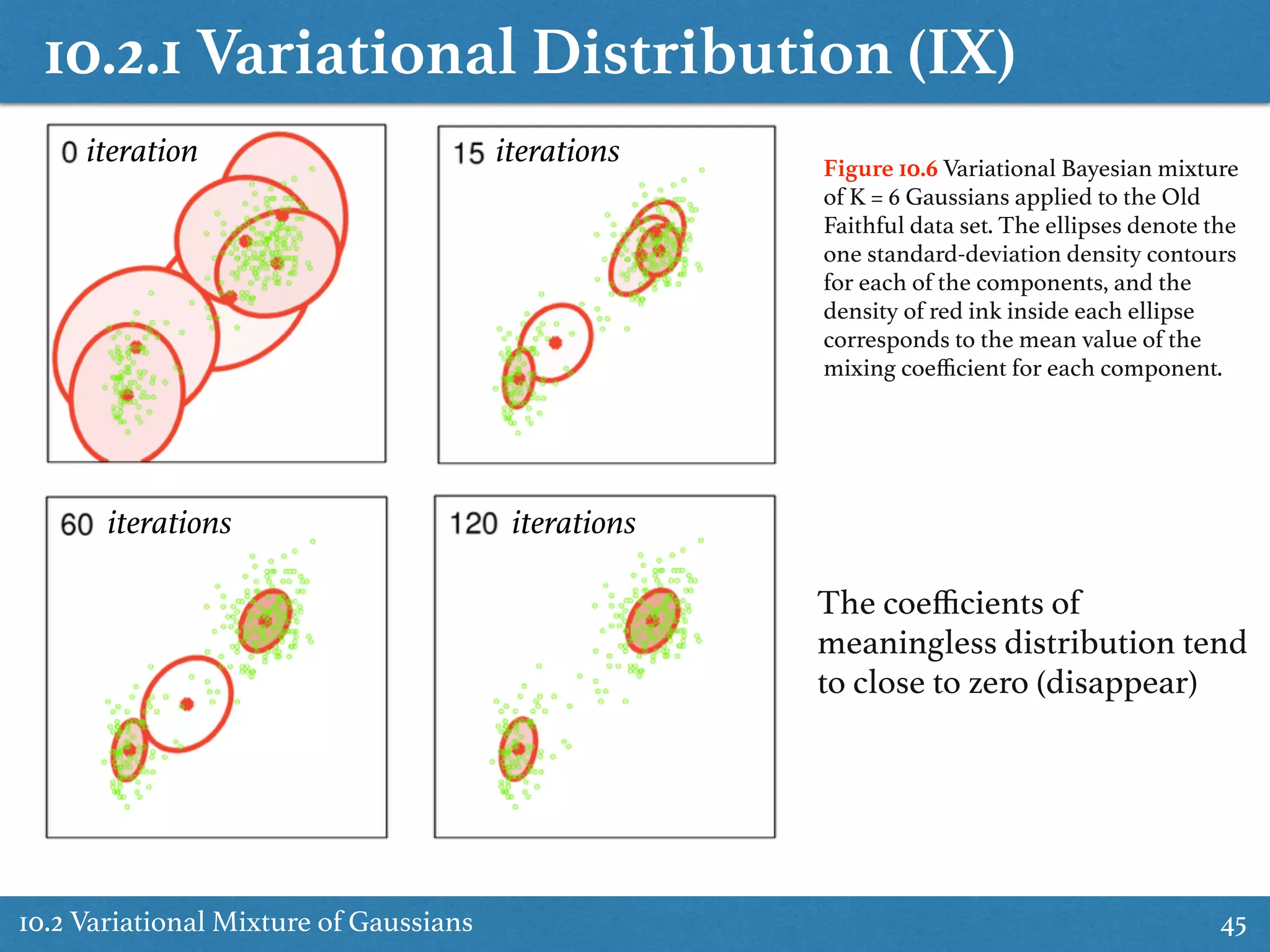
![10.2.1 Variational Distribution (VIII)
10.2 Variational Mixture of Gaussians 44
• Optimize the variational posterior Gaussian mixture distribution
(1) Initialize the responsibilities rnk
(2) Update by (10.51)-(10.53)Nk, ¯xk, Sk
(3) [M step]
• Use (10.57) to find
• Use (10.59) to find
(4) [E step]
• Use (10.64)-(10.66) and (10.46) - (10.49) to update
responsibilities to find
(5) Back to (2) until convergence
q⇤
(⇡)
Use the current
distribution of
parameters to evaluate
responsibilities
Fix responsibilities and
use it to recompute the
variational distribution
over parameters
q⇤
(µk, ⇤k) (k = 1, ..., K)](https://image.slidesharecdn.com/prmlreadingchapter10approximateinference-151228152004/75/Approximate-Inference-Chapter-10-PRML-Reading-44-2048.jpg)
![10.2.5 Induced factorizations
10.2 Variational Mixture of Gaussians 50
Induced factorization arises from an interaction between the factorization
assumption in variational posterior and the conditional independence
properties of the true posterior
• For ex: Let A, B, C be disjoint groups of latent variables
• Factorization assumption
• The optimal solution ln q⇤
(A, B) = EC[ln p(A, B|X, C)] + const
q(A, B, C) = q(A, B)q(C)
• We need to determine if .
This is possible iff
• This can also determined from the directed-graph
model](https://image.slidesharecdn.com/prmlreadingchapter10approximateinference-151228152004/75/Approximate-Inference-Chapter-10-PRML-Reading-50-2048.jpg)
![10.3.1 Variational Distribution
10.3 Variational Linear Regression 54
• Goal: find an approximation to the posterior distribution p(w, ↵|t)
• Factorized approximation
q(w, ↵) = q(w)q(↵) (10.91)
• Optimal solution (from 10.9) ln q⇤
j (Zj) = Ei6=j[ln p(X, Z)] + const
ln q⇤
(↵) = Ew[ln (p(t|w)p(w|↵)p(↵))] + const
= ln p(↵) + Ew[ln p(w|↵)] + const
= (a0 1) ln ↵ b0↵ +
M
2
ln ↵
↵
2
Ew[wT
w] + const
(10.92)
then
q⇤
(↵) = Gam(↵|aN , bN ) where(10.93)
(10.94)
(10.95)
M is number of fitting
parameters wi or input
dimension](https://image.slidesharecdn.com/prmlreadingchapter10approximateinference-151228152004/75/Approximate-Inference-Chapter-10-PRML-Reading-54-2048.jpg)
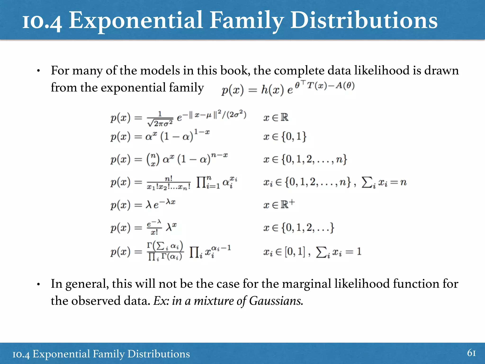
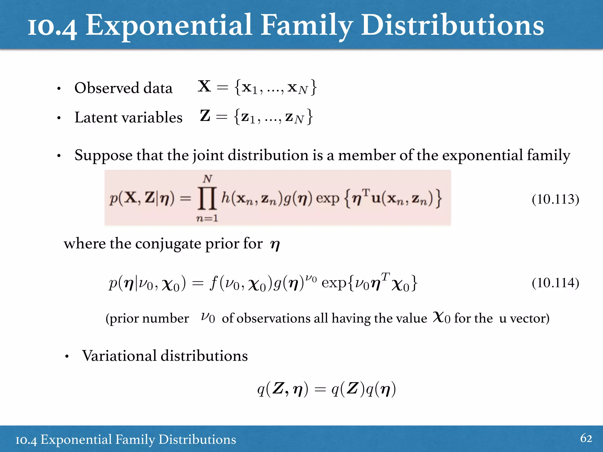
![10.4 Exponential Family Distributions
10.4 Exponential Family Distributions 63
ln q⇤
j (Zj) = Ei6=j[ln p(X, Z)] + const• Optimal solution (from 10.9)
= E⌘[ln p(X, Z|⌘)] + const
=
NX
n=1
ln h(xn, zn) + E⌘[⌘T
]u(xn, zn) + const
sum of independent things
Induced factorization
q⇤
(Z) =
Y
n
q⇤
(zn)
(10.115)
where
(10.116)
ln q⇤
(Z) = E⌘[ln p(X, Z, ⌘)] = E⌘[ln p(X, Z|⌘)p(⌘|⌫0, 0)p(⌫0, 0)]
q⇤
(zn) = h(xn, zn)g(E⌘[⌘]) exp{E⌘[⌘T
]u(xn, zn)}](https://image.slidesharecdn.com/prmlreadingchapter10approximateinference-151228152004/75/Approximate-Inference-Chapter-10-PRML-Reading-63-2048.jpg)
![10.4 Exponential Family Distributions
10.4 Exponential Family Distributions 64
ln q⇤
j (Zj) = Ei6=j[ln p(X, Z)] + const• Optimal solution (from 10.9)
ln q⇤
(⌘) = EZ[ln p(X, Z, ⌘)] = EZ[ln p(X, Z|⌘)p(⌘|⌫0, 0)p(⌫0, 0)]
= ln p(⌘|⌫0, 0) + EZ[ln p(X, Z|⌘)] + const
= ⌫0 ln g(⌘) + ⌫0⌘T
0 +
NX
n=1
ln g(⌘) + ⌘T
Ezn [u(xn, zn)] + const
(10.118)
q⇤
(⌘) = f(⌫N , N )g(⌘)⌫N
exp{⌫N ⌘T
N }
then
where
(10.119)
(10.120)
(10.121)](https://image.slidesharecdn.com/prmlreadingchapter10approximateinference-151228152004/75/Approximate-Inference-Chapter-10-PRML-Reading-64-2048.jpg)
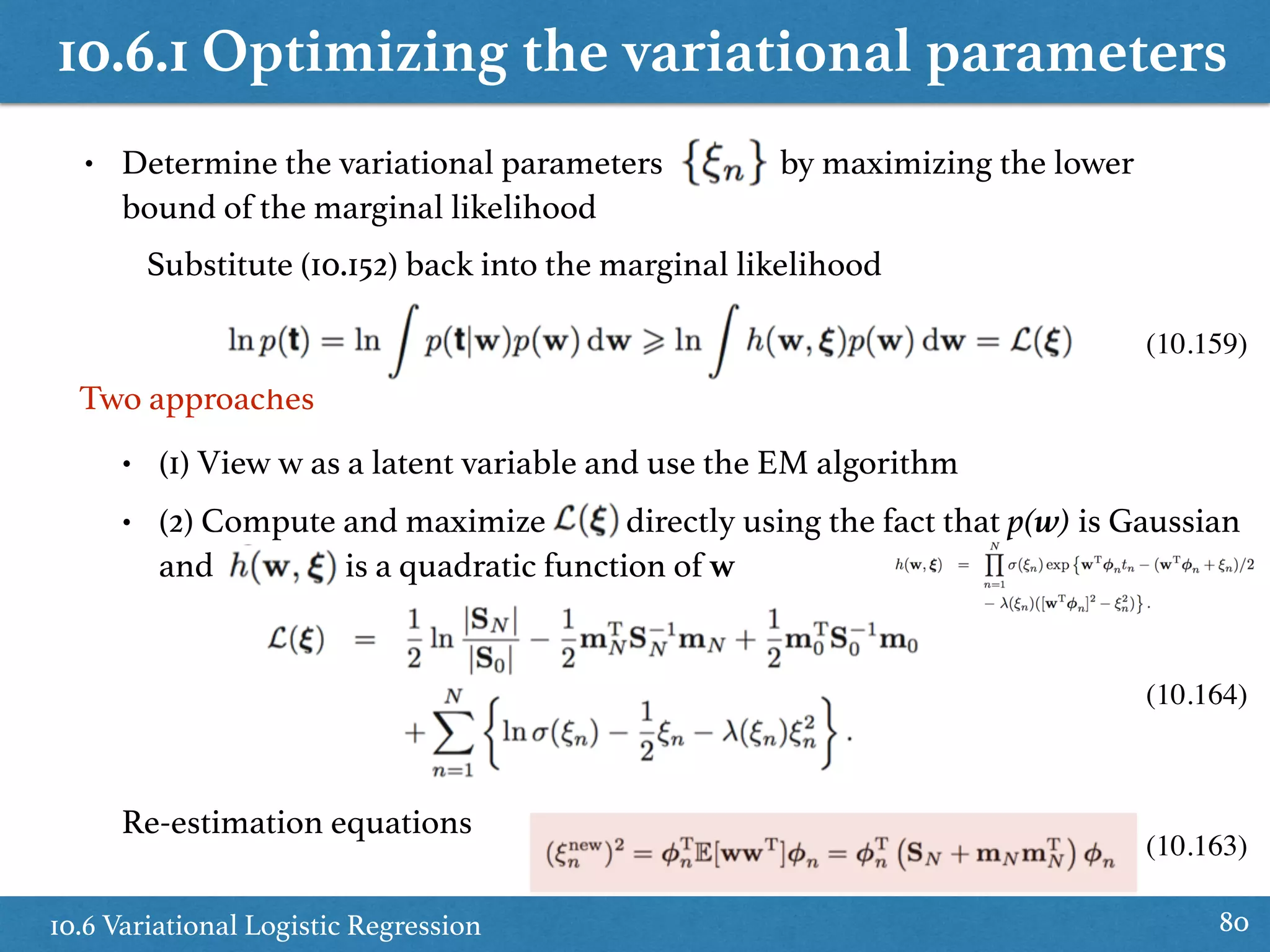
![10.6.1 Optimizing the variational parameters
10.6 Variational Logistic Regression 81
• Invoke EM algorithm
1. Initialize values for
2. E step
• Use to calculate the posterior distribution
3. M step
⇠old
• Maximize the complete-data log likelihood
Q(⇠, ⇠old
) = Eq(w) [ln h(w, ⇠)p(w)]
• Solve (stationarity condition)
then (10.163)
(10.160)
(10.162)](https://image.slidesharecdn.com/prmlreadingchapter10approximateinference-151228152004/75/Approximate-Inference-Chapter-10-PRML-Reading-81-2048.jpg)
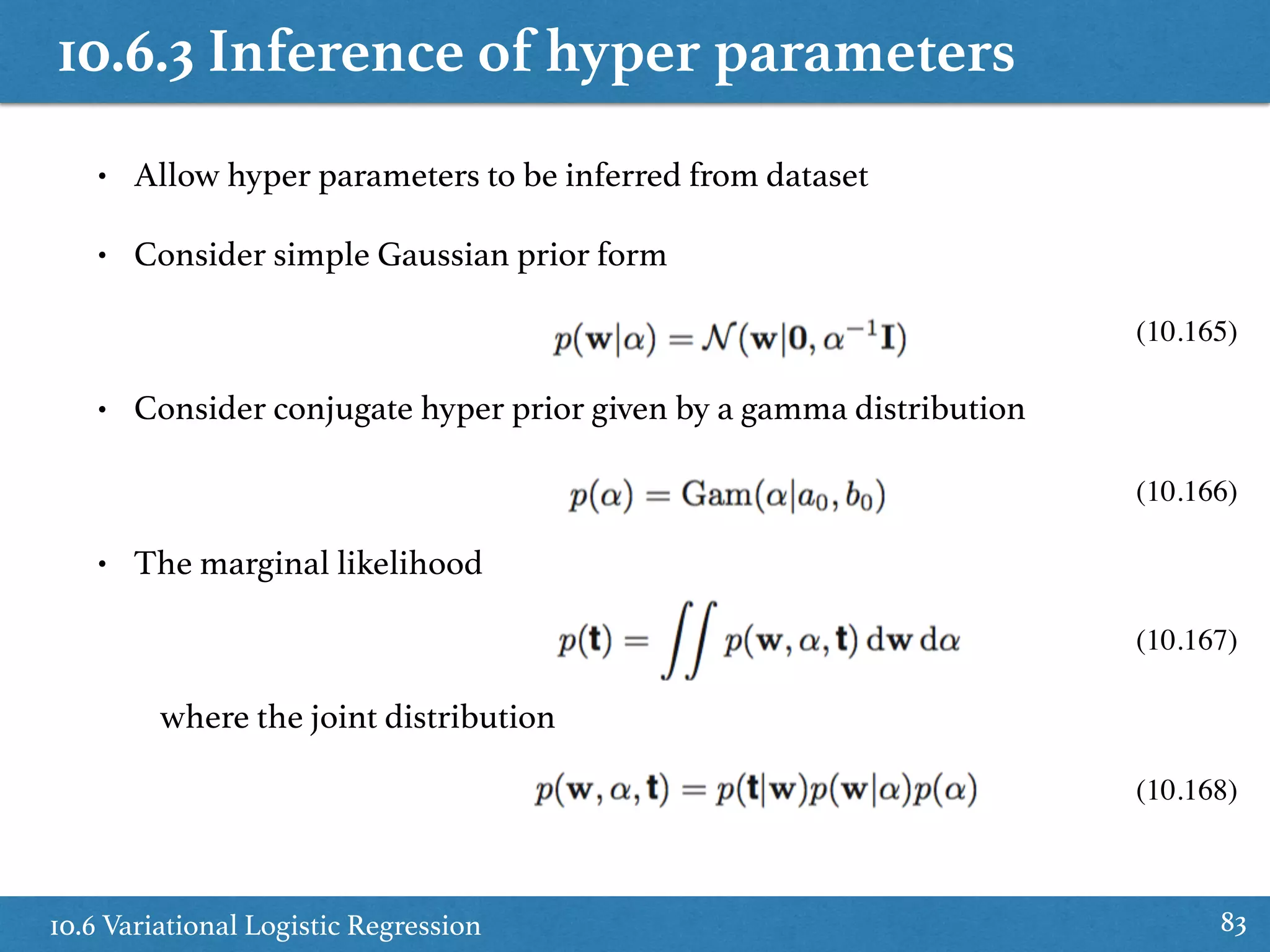
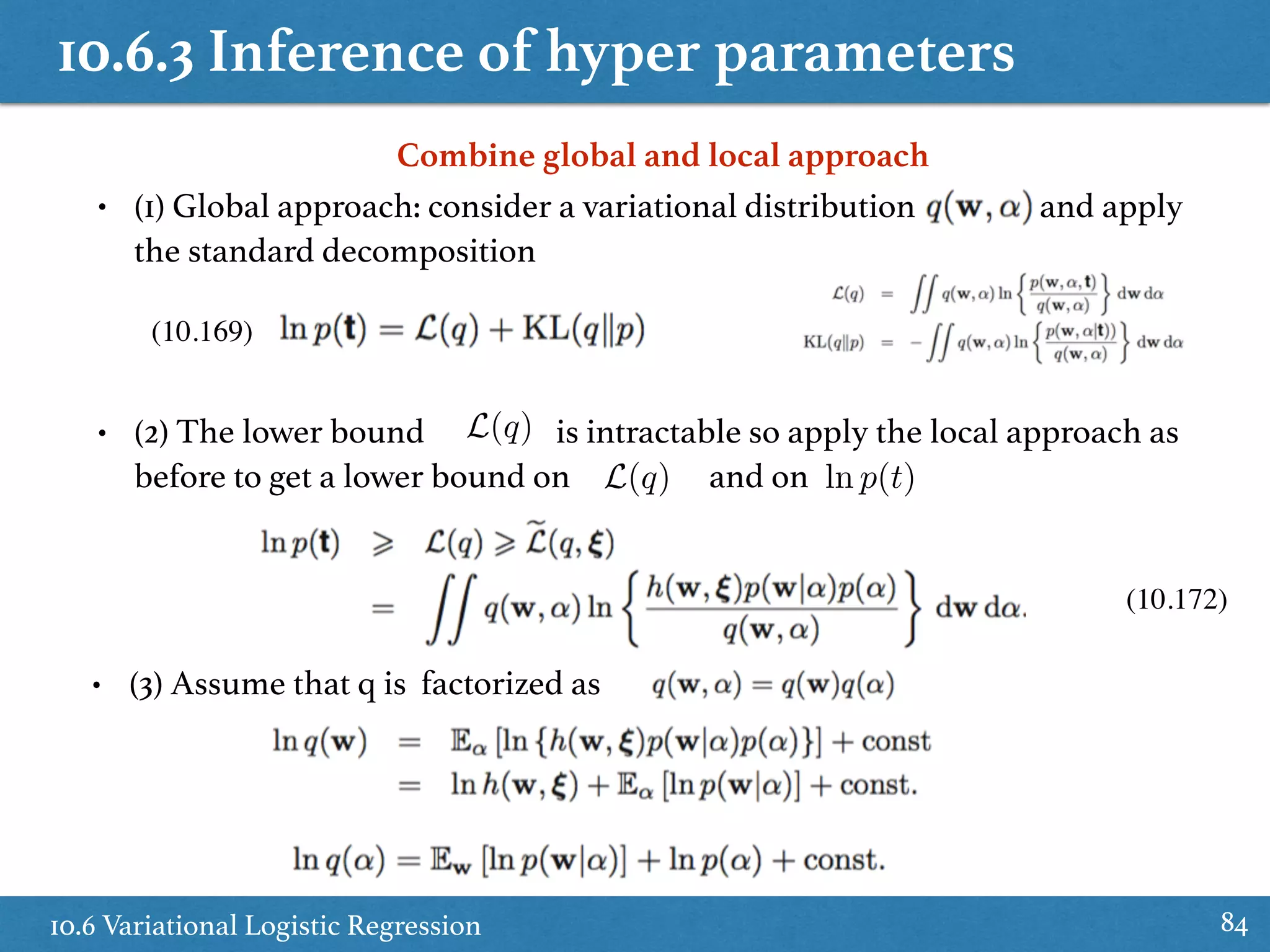
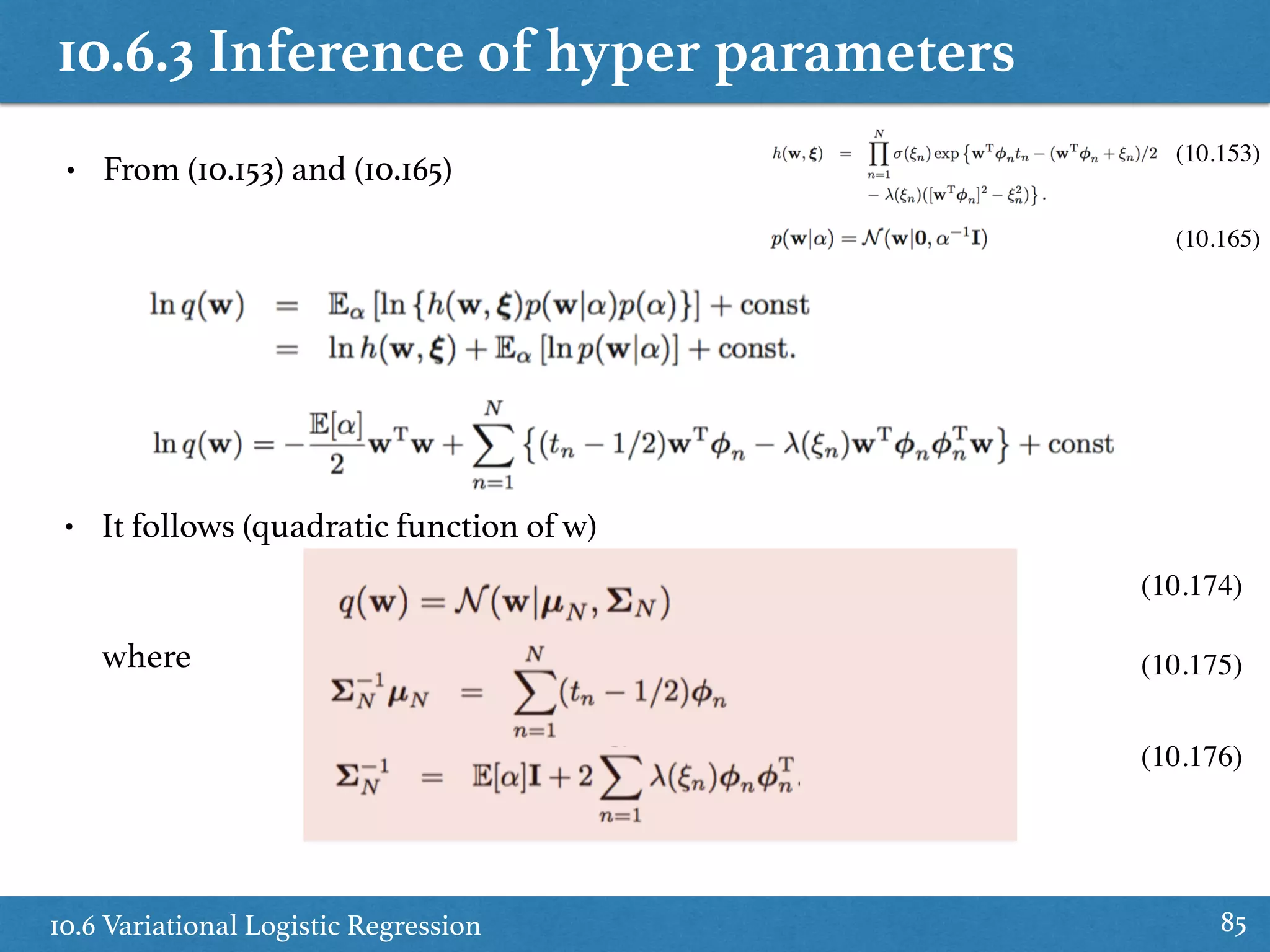
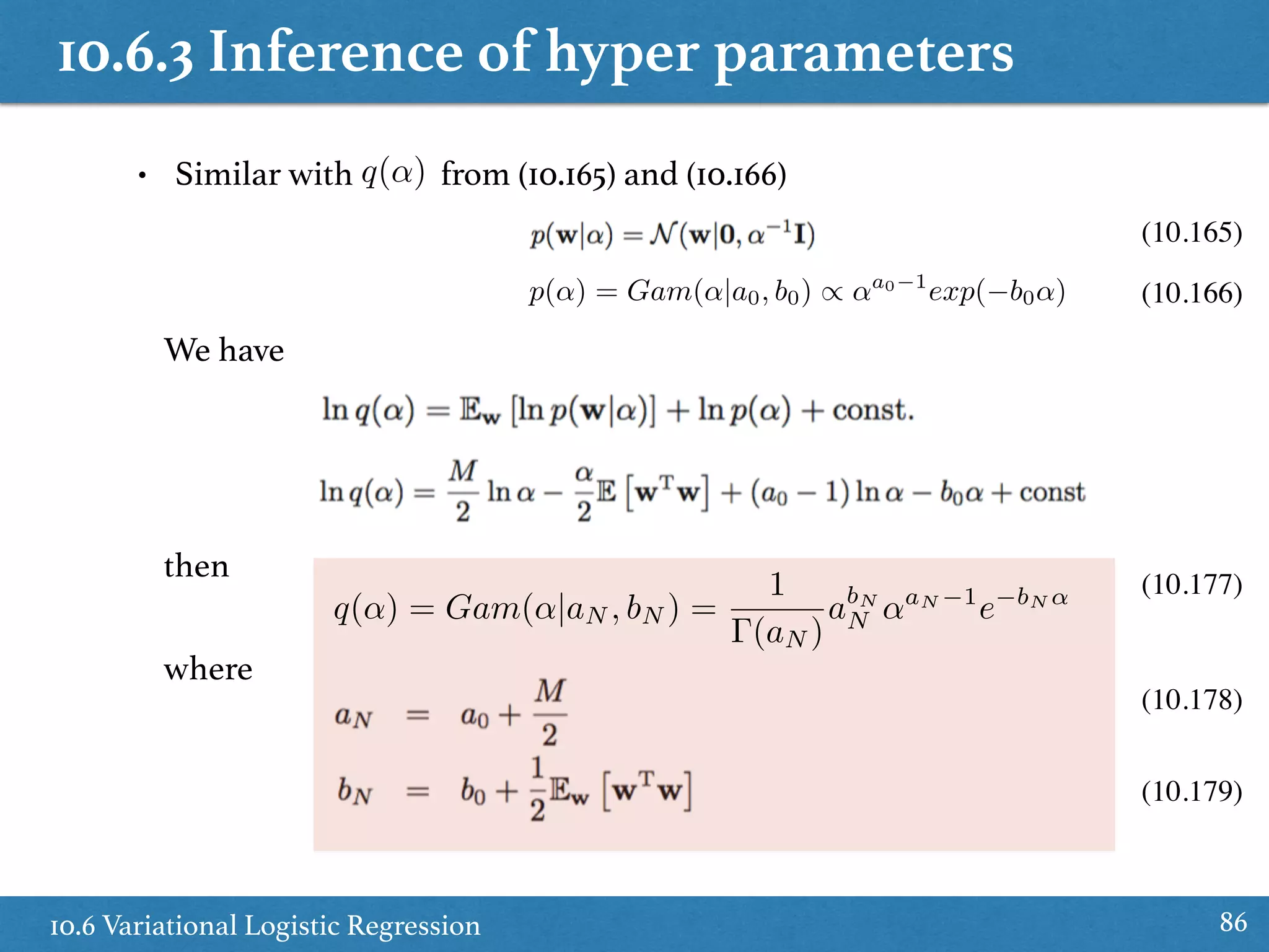
![10.6.3 Inference of hyper parameters
10.6 Variational Logistic Regression 87
• The variational parameters are obtained by maximizing the lower bound
(10.180)
(10.181)
(10.183)
(10.182)
• Re-estimation equations
where
Q(⇠, ⇠old
) = Eq(w) [ln h(w, ⇠)p(w)] (10.160)
as we done before with](https://image.slidesharecdn.com/prmlreadingchapter10approximateinference-151228152004/75/Approximate-Inference-Chapter-10-PRML-Reading-87-2048.jpg)

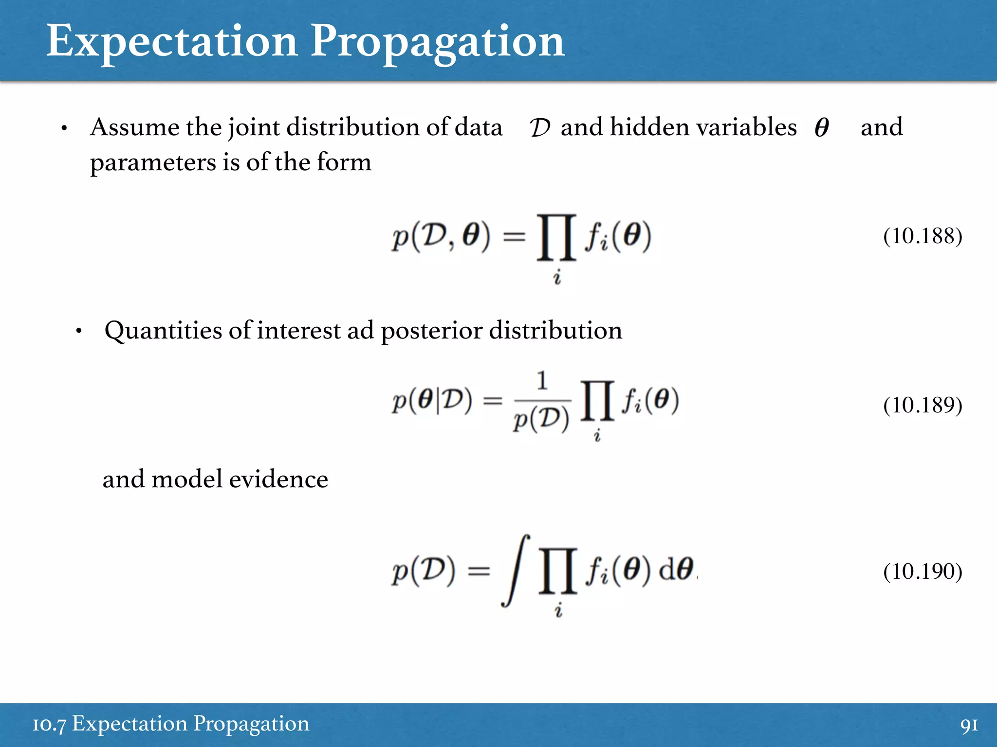
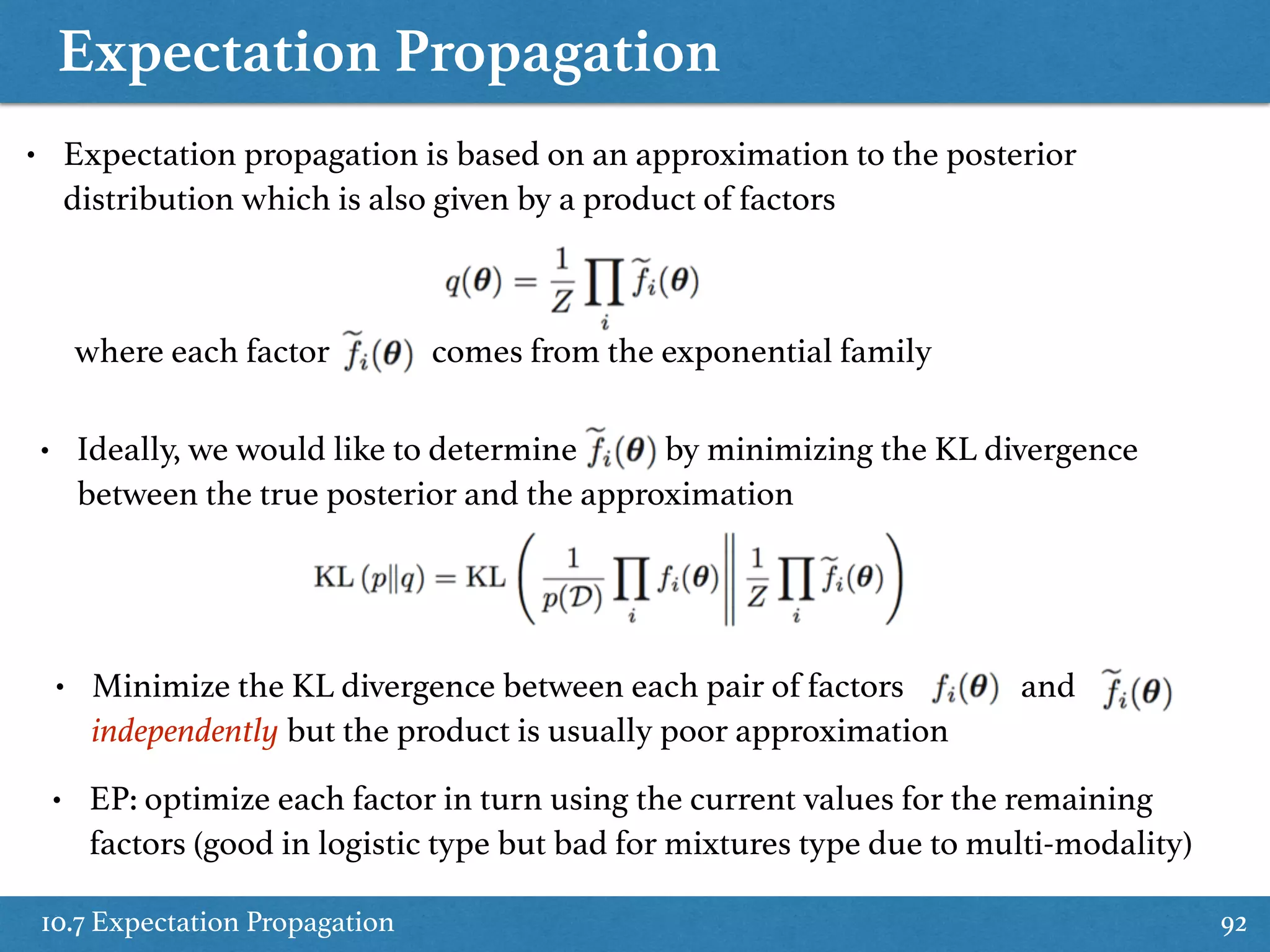
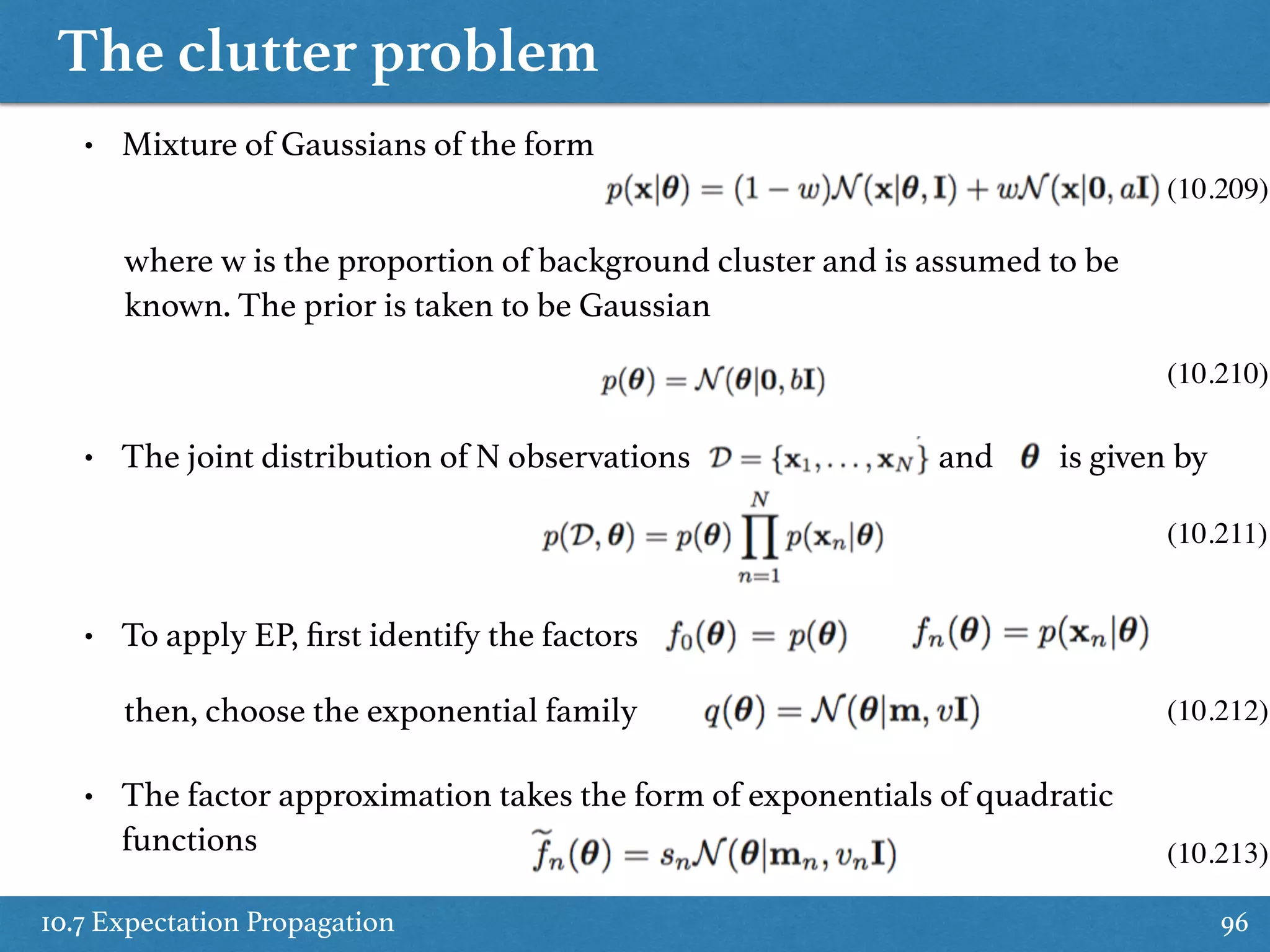
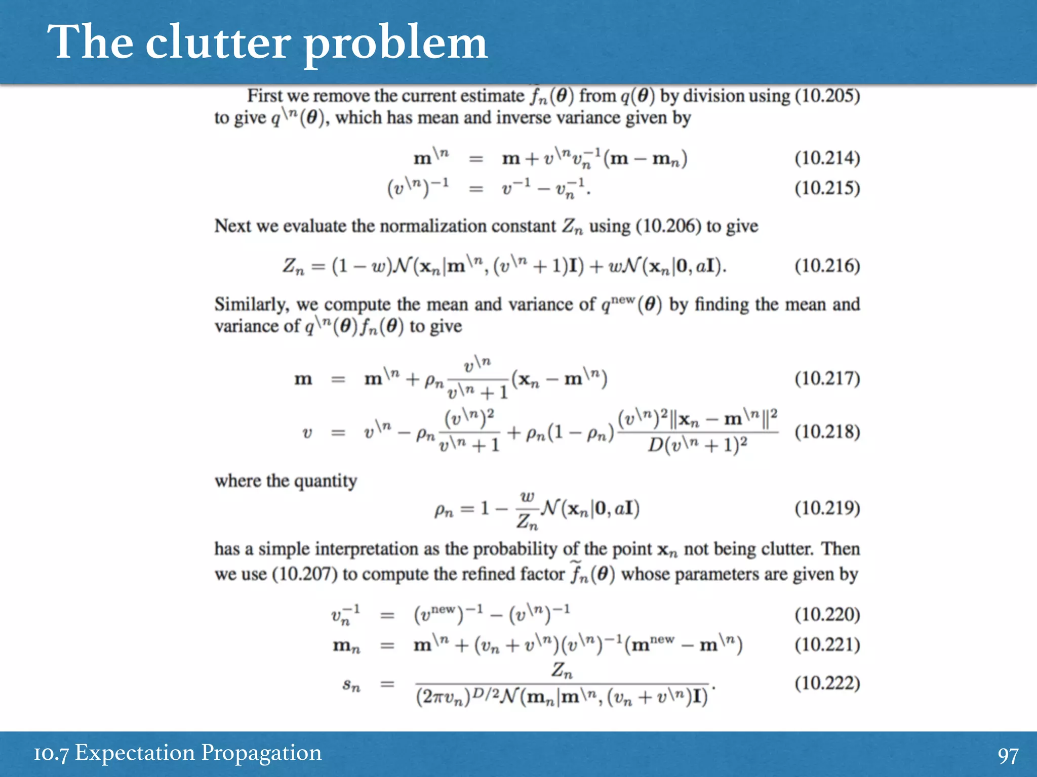
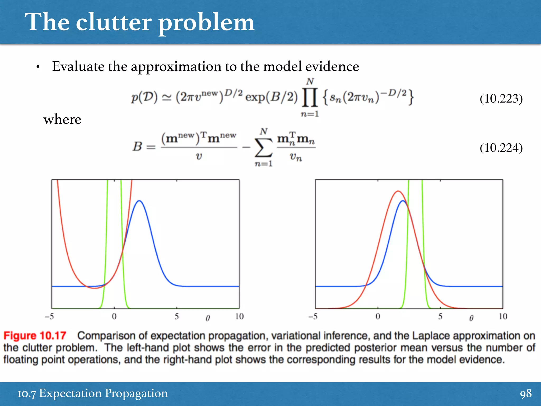
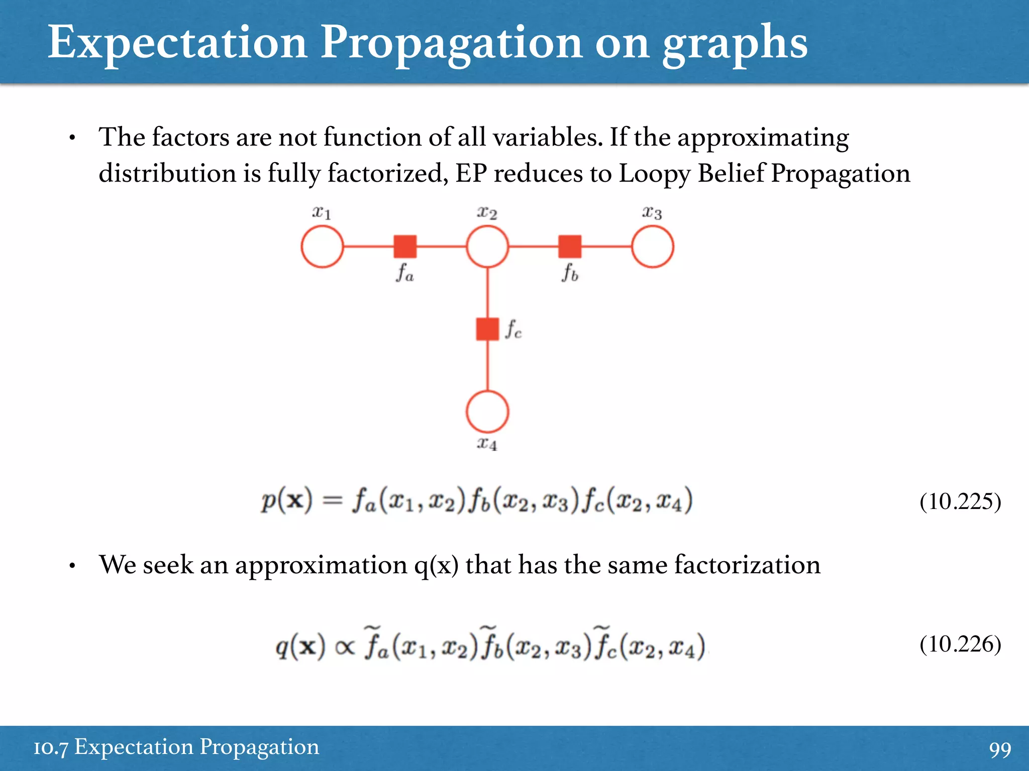
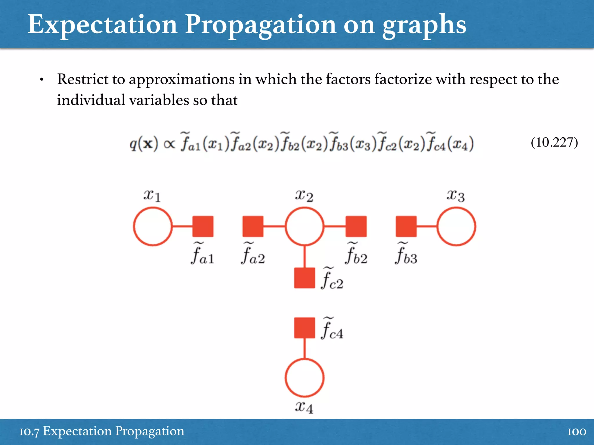
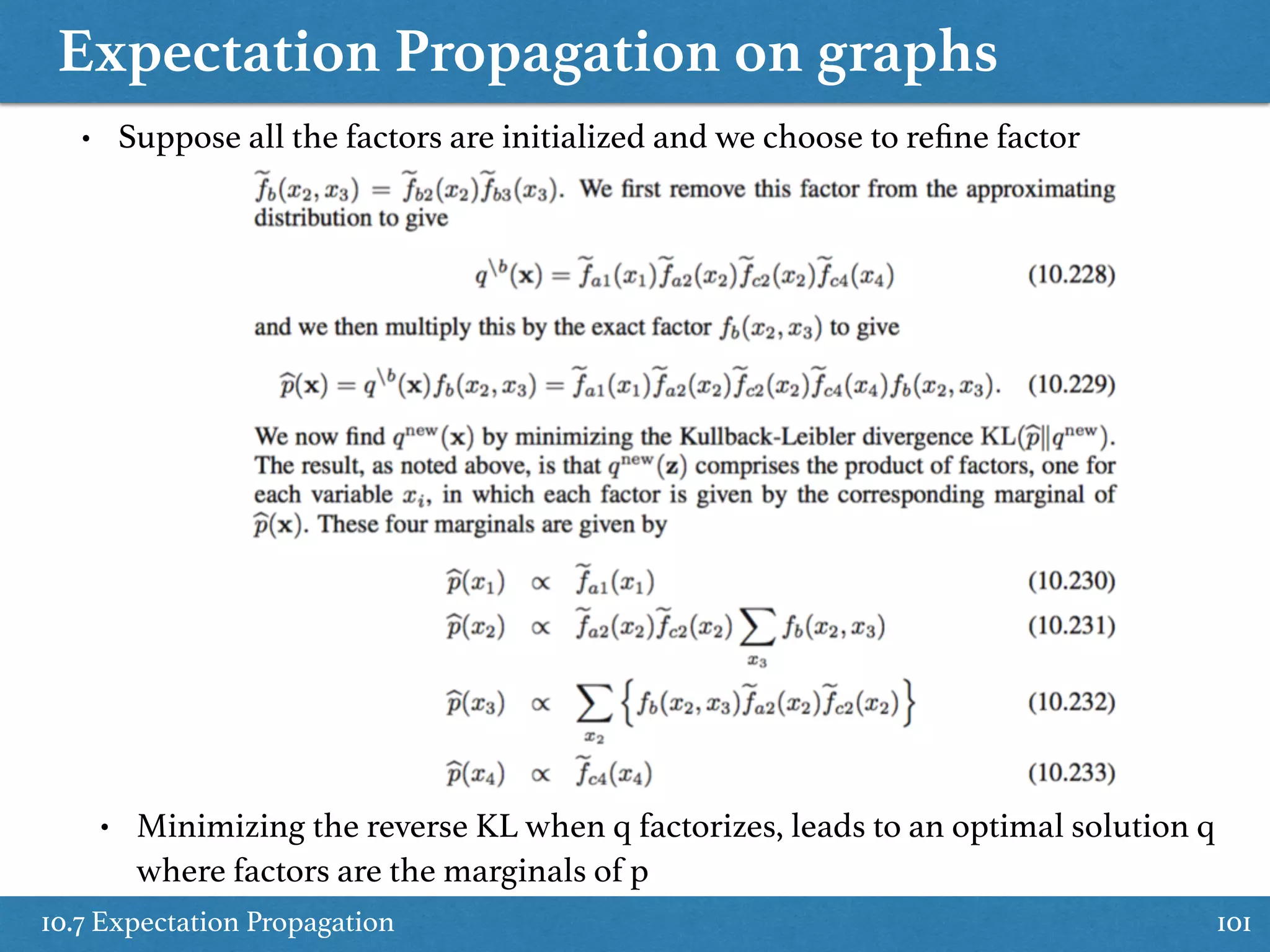
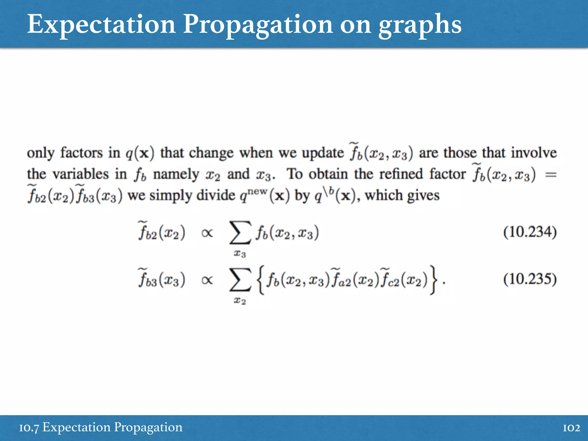
![Expectation Propagation (Minka, 2001)
10.7 Expectation Propagation 89
• An alternative form of deterministic approximate inference based on the
reverse KL divergence KL(p||q) ( instead of KL(q||p)) where p is the complex
distribution
KL(p||q) =
Z
p(z) ln
p(z)
q(z)
dzKL(q||p) =
Z
q(z) ln
q(z)
p(z)
dz
• Consider fixed distribution p(z) and member of the exponential family q(z).
KL(p||q) = ln g(⌘) ⌘T
Ep(z)[u(z)] + const
⌘
setting gradient to zero
(10.185)
(10.186)
q(z) = h(z)g(⌘) exp{⌘T
u(z)}
• The Kullback-Leibler divergence as function of
(10.184)](https://image.slidesharecdn.com/prmlreadingchapter10approximateinference-151228152004/75/Approximate-Inference-Chapter-10-PRML-Reading-89-2048.jpg)
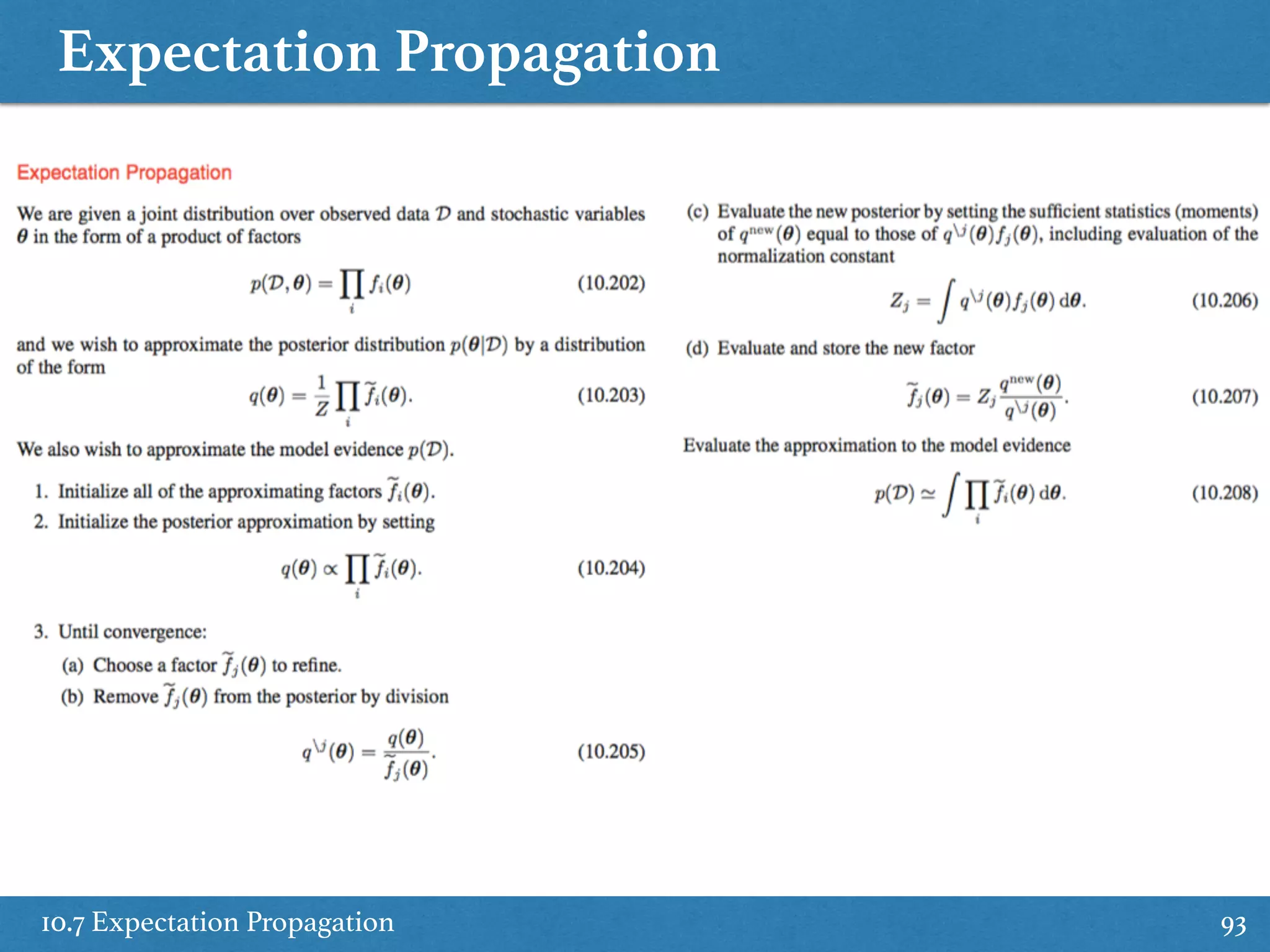
![Expectation Propagation
10.7 Expectation Propagation 90
• Member of the exponential family q(z).
(10.187)
q(z) = h(z)g(⌘) exp{⌘T
u(z)} (10.184)
then Z
h(z)g(⌘) exp{⌘T
u(z)}dz = 1
taking the gradient of both size
rg(⌘)
Z
h(z) exp{⌘T
u(z)}dz +g(⌘)
Z
h(z) exp{⌘T
u(z)}u(z)dz = 0
1
g(⌘)
rg(⌘) = g(⌘)
Z
h(z) exp{⌘T
u(z)}u(z)dz = Eq(z)[u(z)]
r ln g(⌘) = Eq(z)[u(z)]
From 10.186 we have
Moment matching, setting mean and covariance of q(z) the same as p(z)’s](https://image.slidesharecdn.com/prmlreadingchapter10approximateinference-151228152004/75/Approximate-Inference-Chapter-10-PRML-Reading-90-2048.jpg)


The document summarizes key concepts from Chapter 10 of Bishop's PRML book on approximate inference using variational methods. It introduces variational inference as a deterministic alternative to importance sampling for approximating intractable distributions. Variational inference frames inference as an optimization problem of variationally approximating the true posterior using a simpler distribution from an assumed family. This is done by maximizing a lower bound on the marginal likelihood. Mean-field variational inference further assumes a factorized form for the variational distribution.
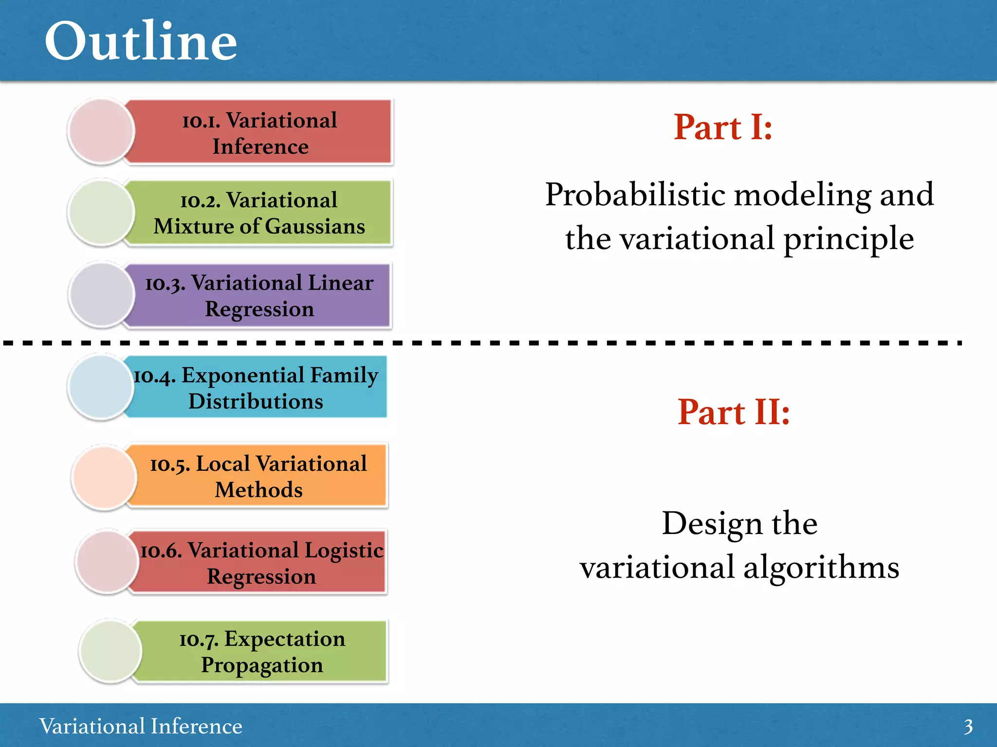
Introduction to Variational Inference from VC.M. Bishop's PRML, detailing the presentation outline and topics.
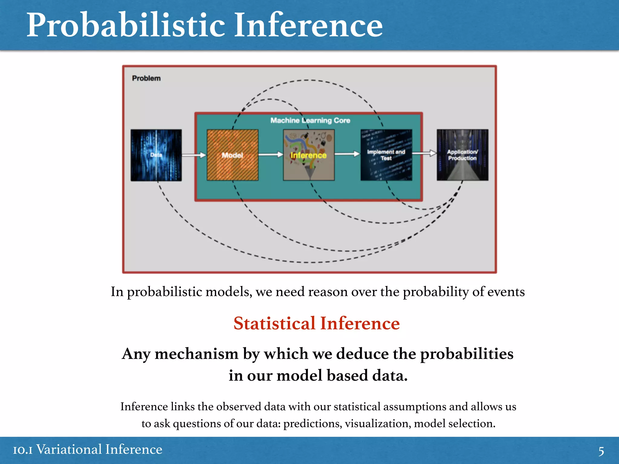
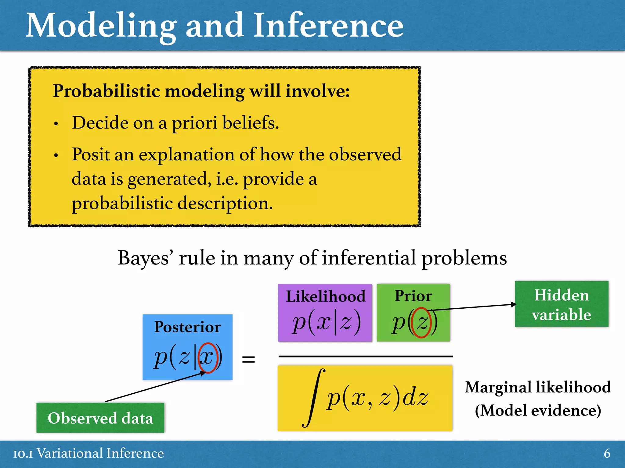
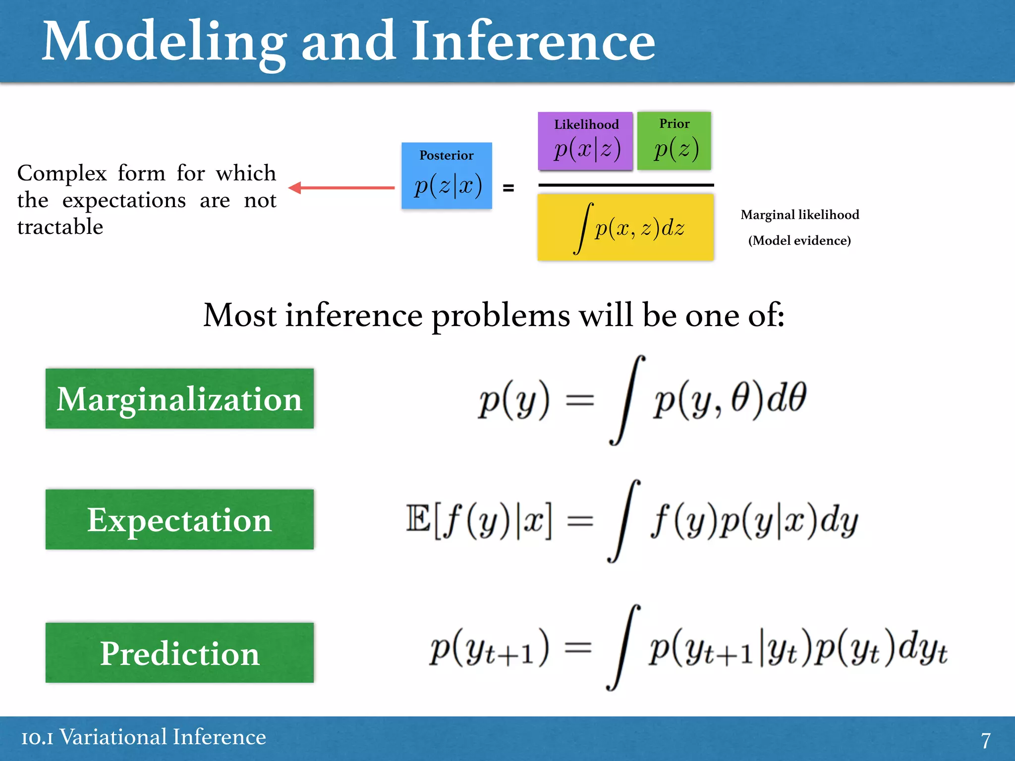
Covers concepts of Probabilistic Inference including Bayes' rule, marginalization, and statistical assumptions.
Explains the idea of importance sampling for estimating expectations and transitioning to variational inference.
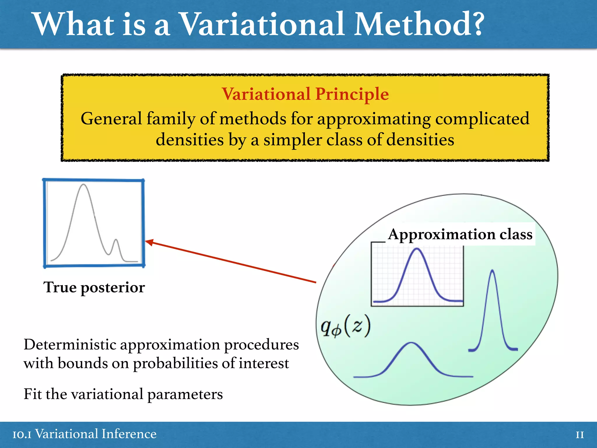
Discussion on variational methods used for approximating densities, including variational calculus and approximation classes.
Describes how to obtain variational lower bounds and the transition from IS to variational inference.
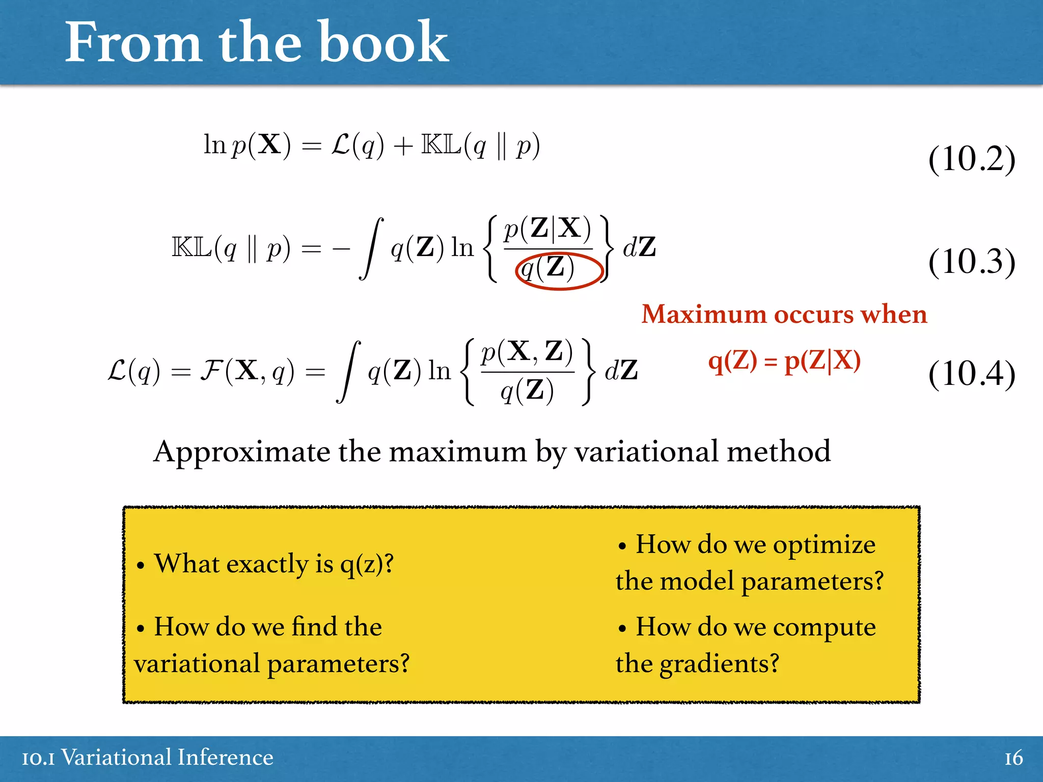
Focus on optimizing variational parameters and deriving KL divergence relationships in variational inference.
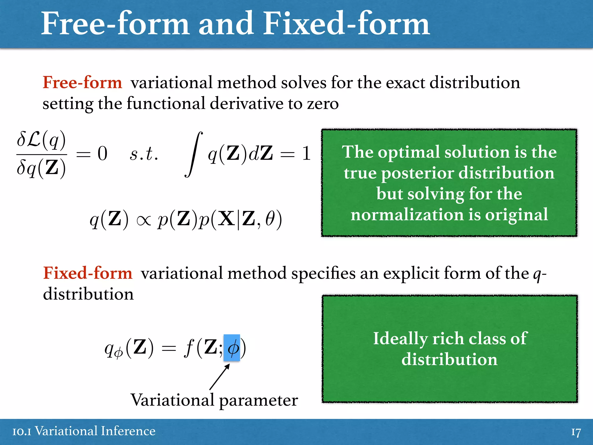
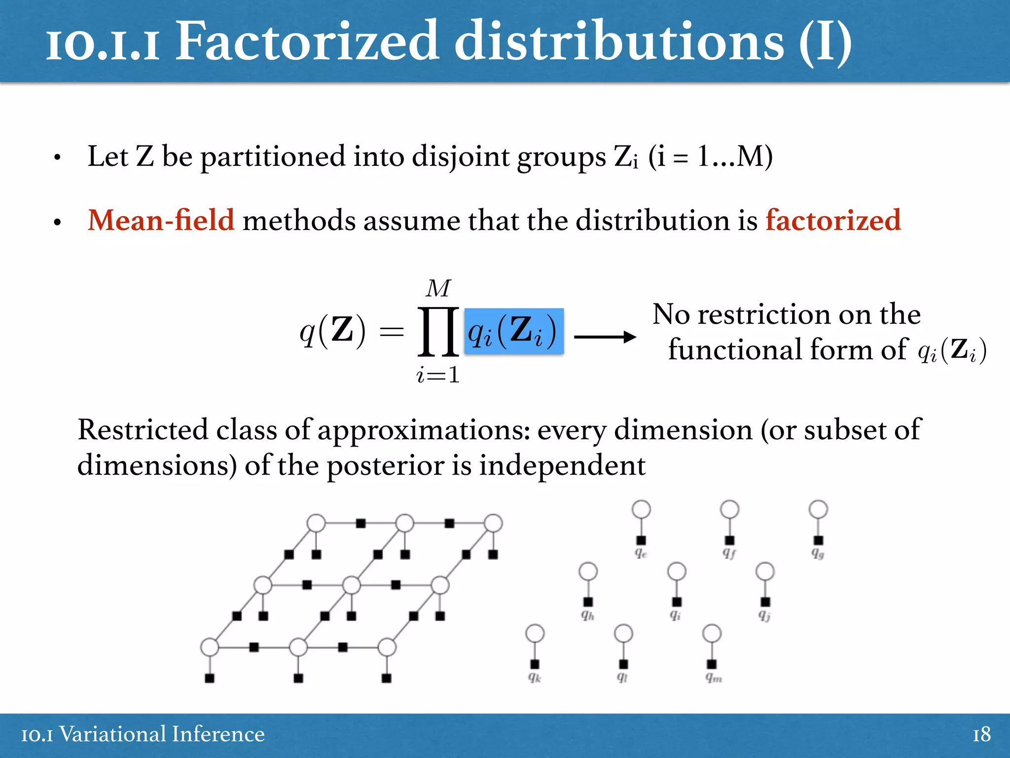
Details on free-form vs fixed-form methods and the concept of factorized distributions in variational inference.
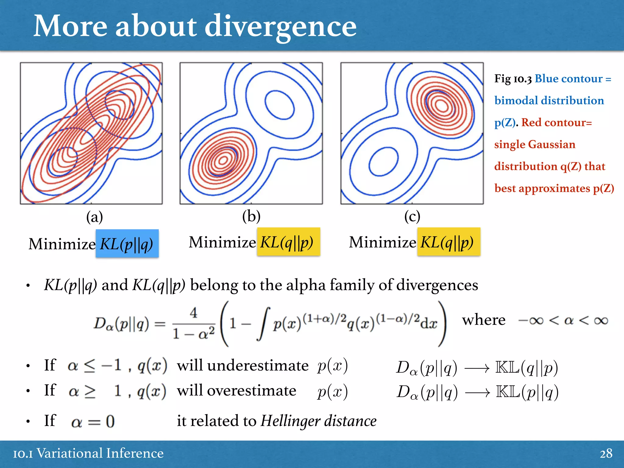
Examines properties and implications of using factorized approximations and KL divergences in modeling.
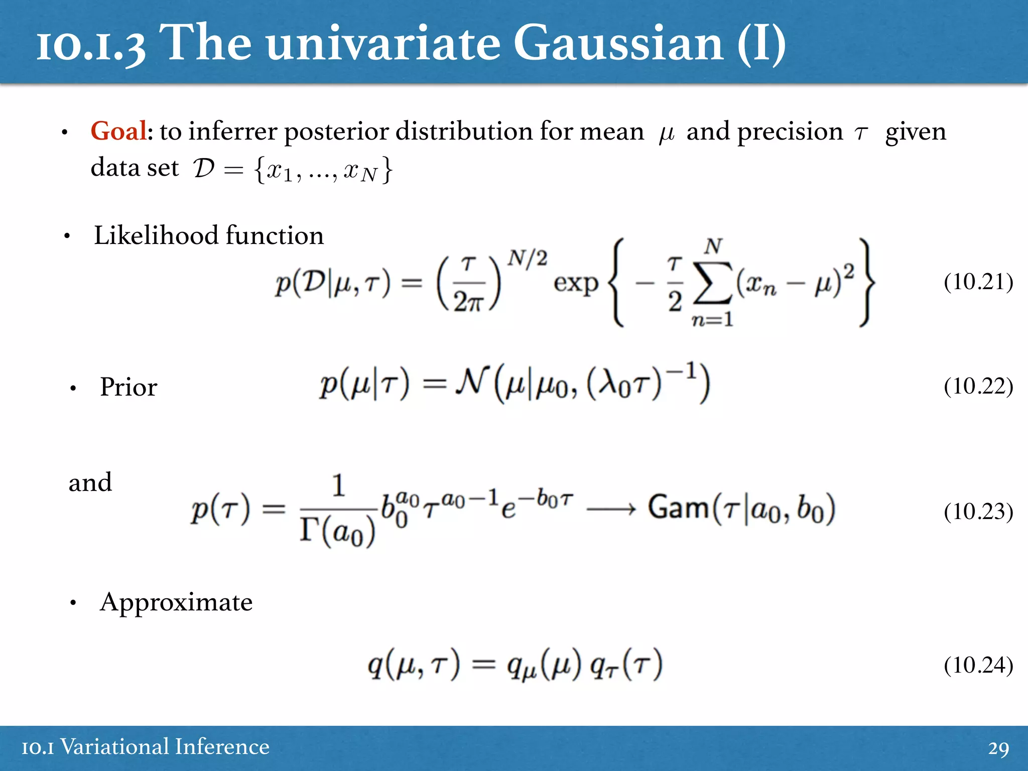
Explains the univariate Gaussian case in variational inference, detailing optimal solutions and posterior distributions.
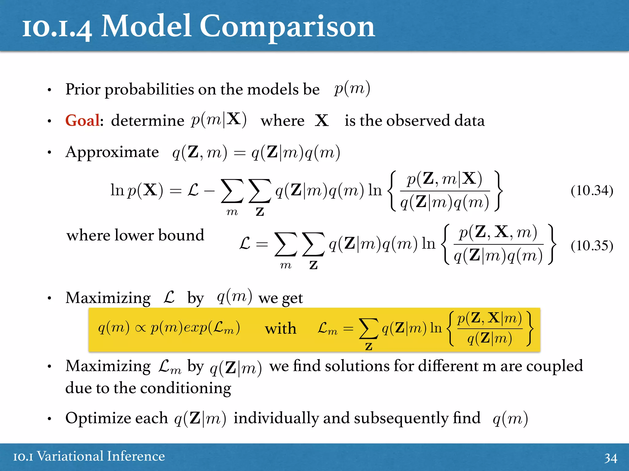
Discusses model comparisons using approximate methods with variational inference techniques, introducing Gaussian mixtures.
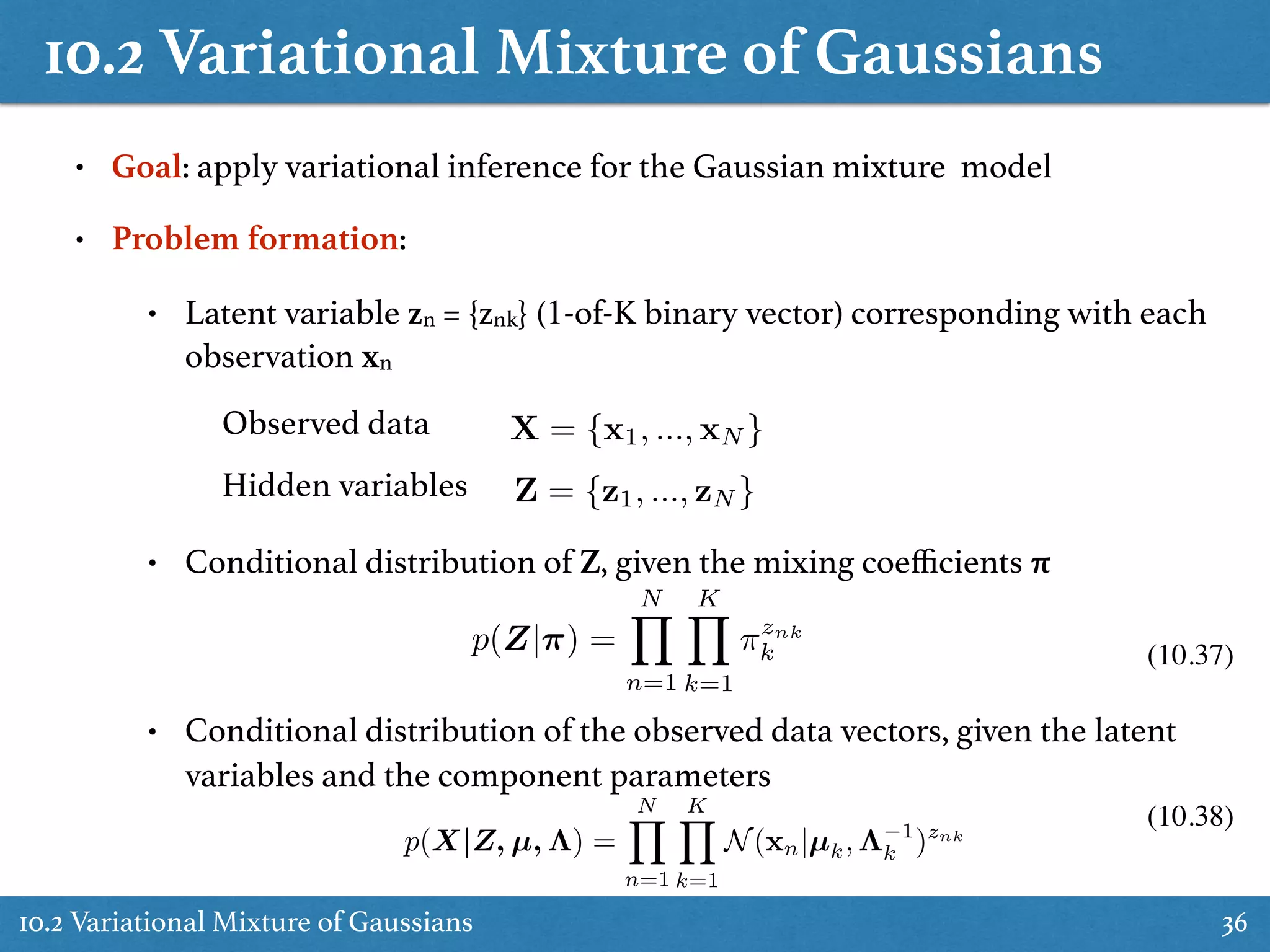
Application of variational inference to Gaussian mixture models, detailing formulations and optimal solutions.
Expands on optimizing variational distributions and predictive density in Gaussian mixtures, discussing convergence.
Discusses the implications of induced factorizations in posterior distributions using variational methods.
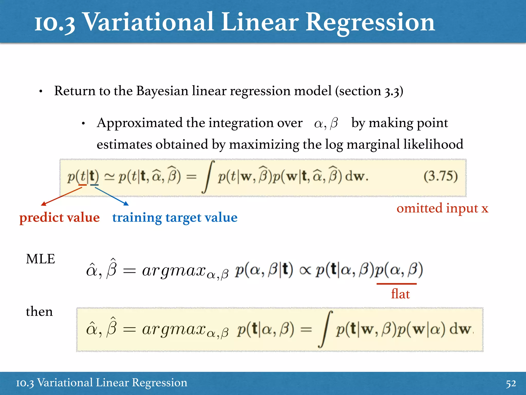
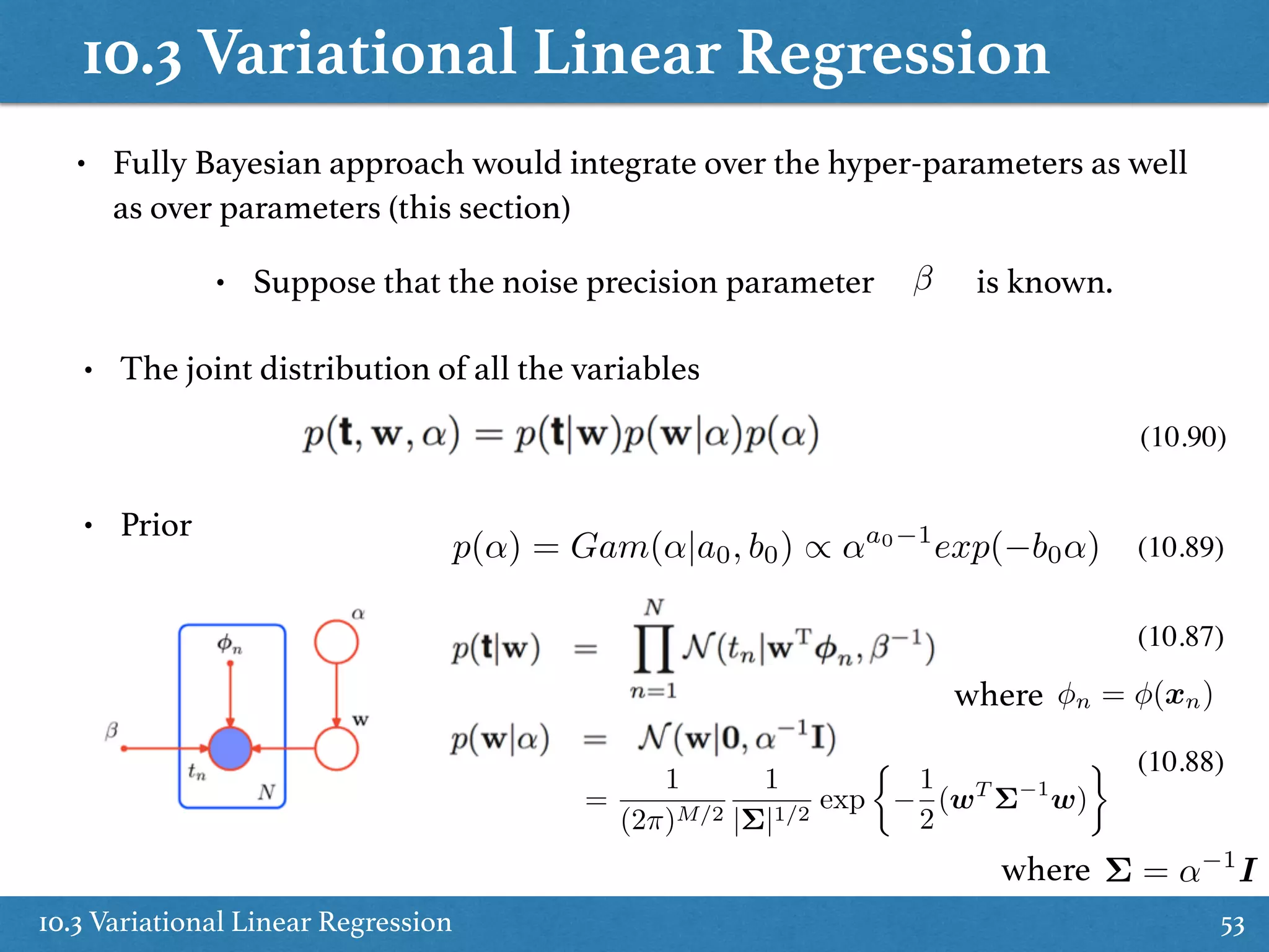
Returns to Bayesian linear regression and sets foundation for variational approximations in this context.
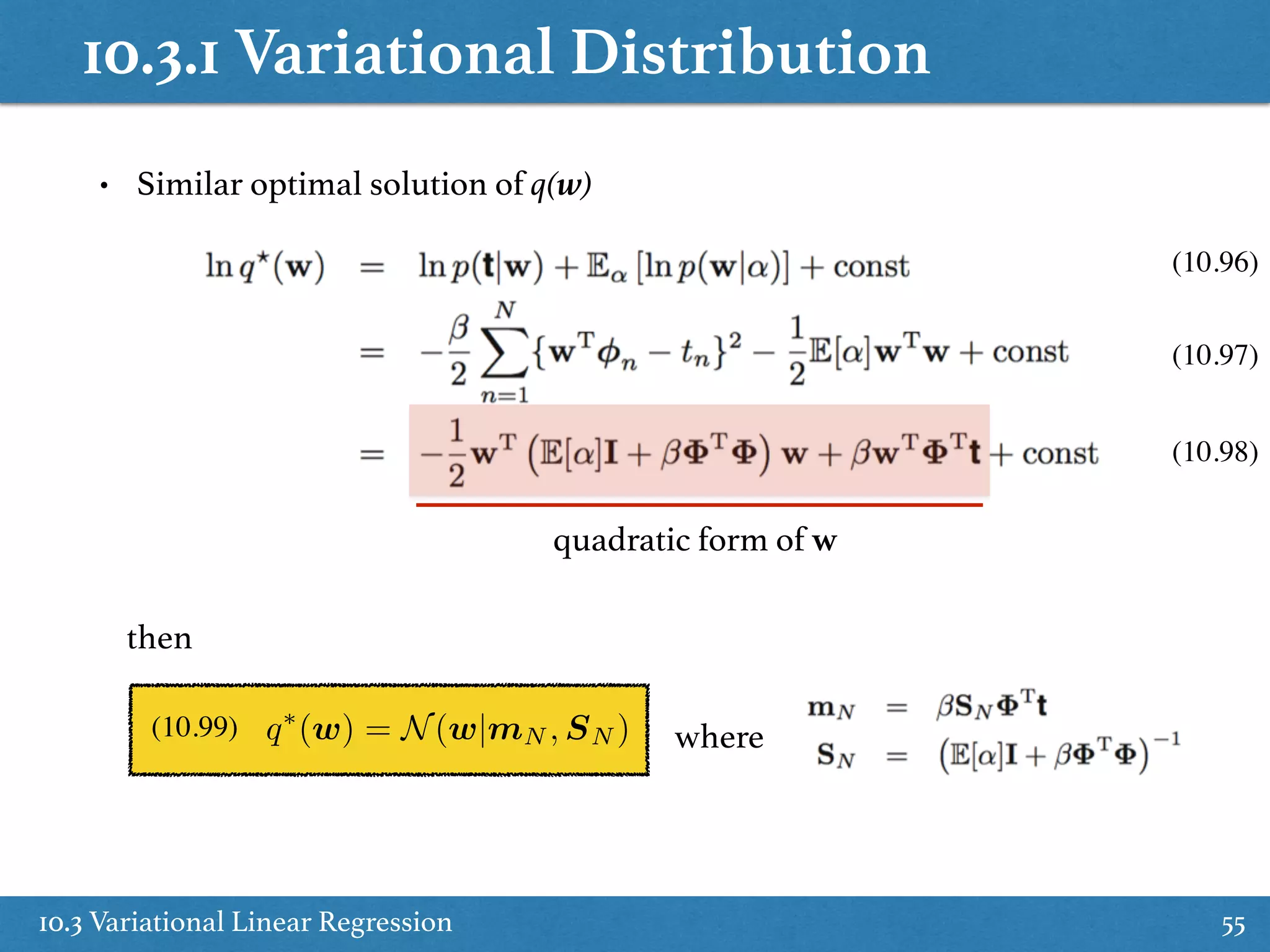
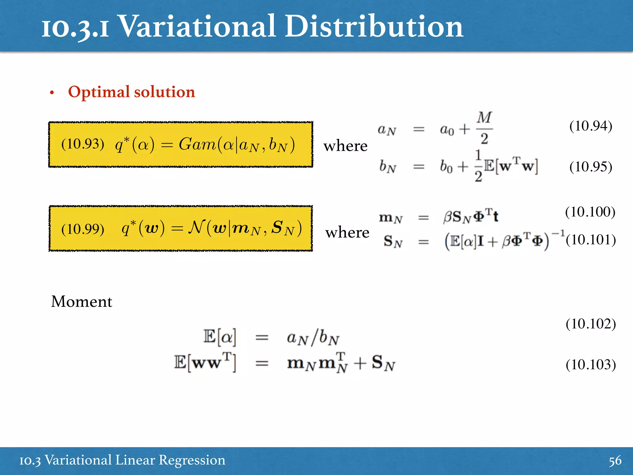
Finds approximations to posterior distributions in Bayesian linear regression, detailing optimal solutions.
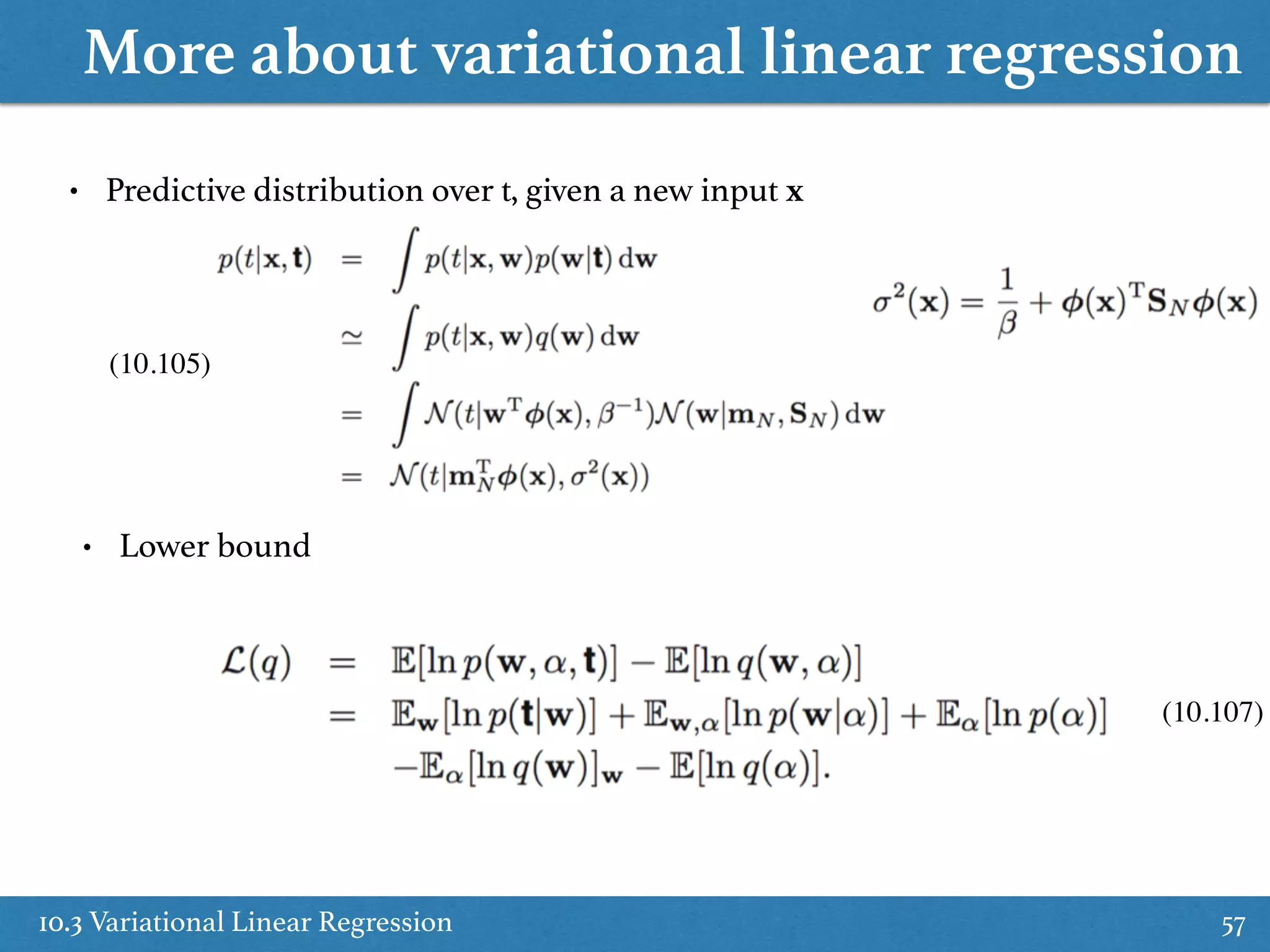
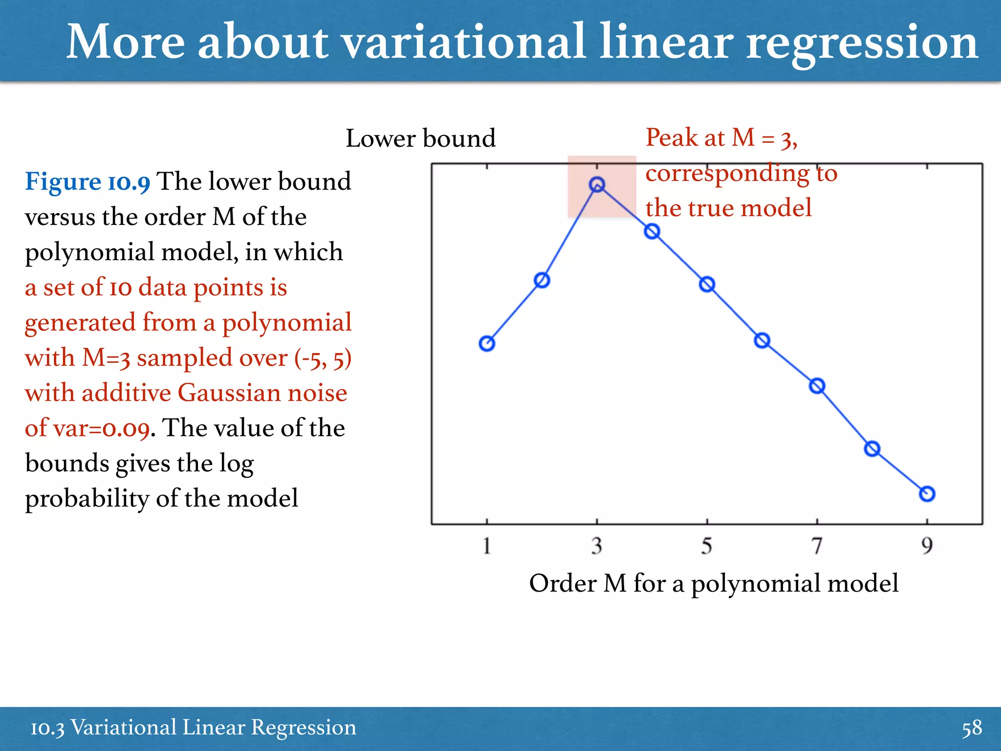
Analysis of predictive distributions and lower bounds concerning linear regression models.
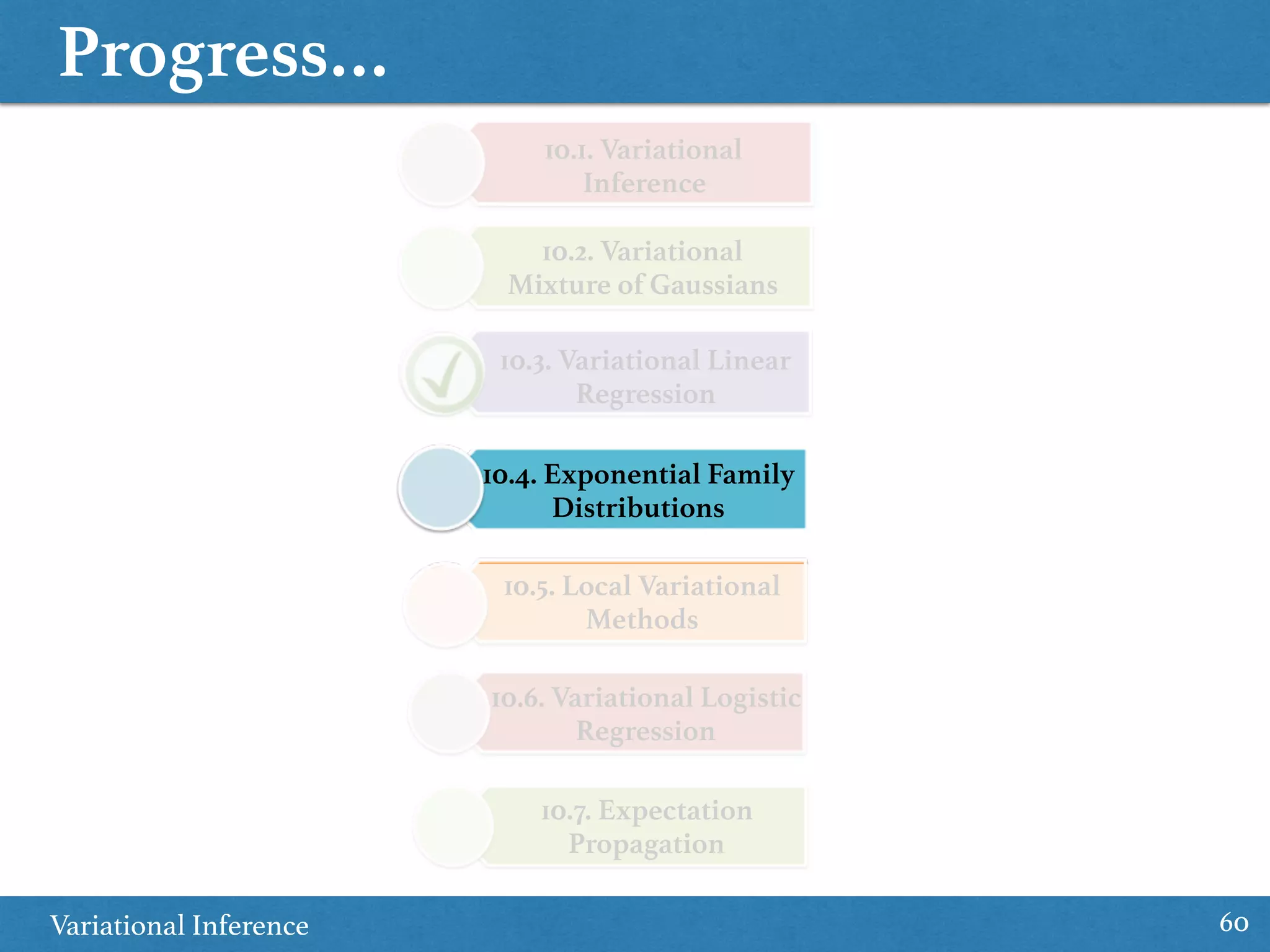
Focus on exponential family distributions and their implications in variational inference methods.
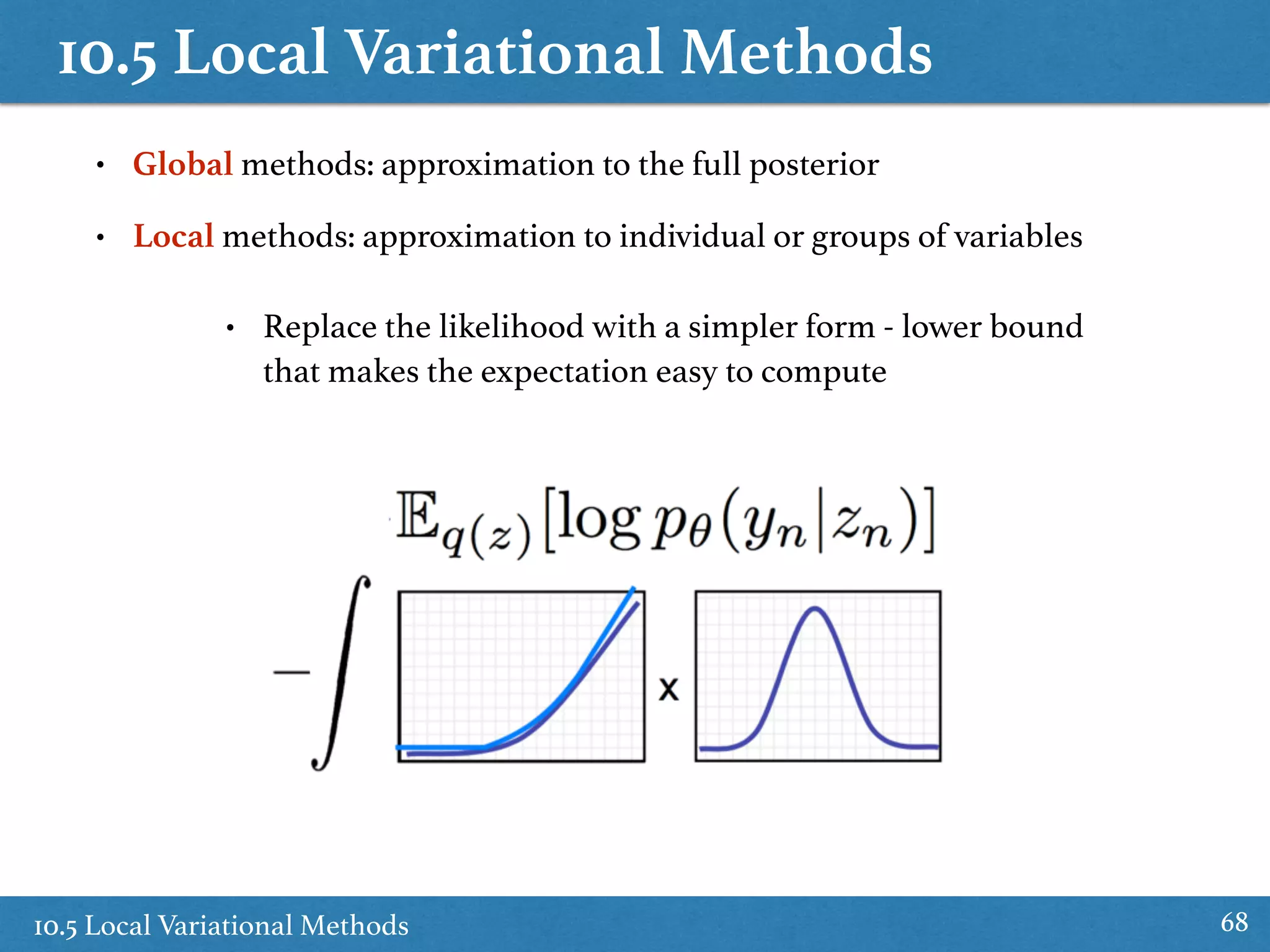
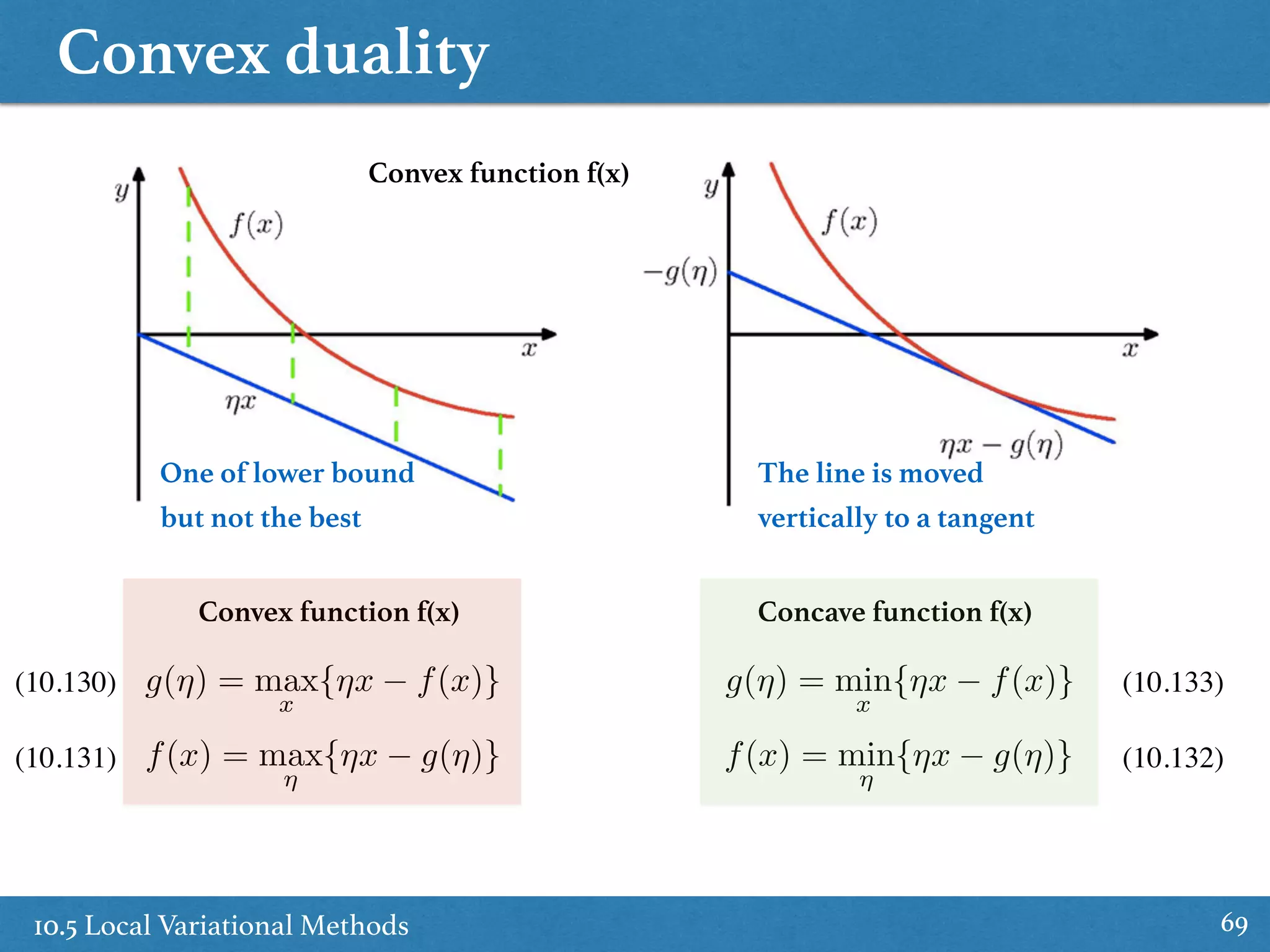
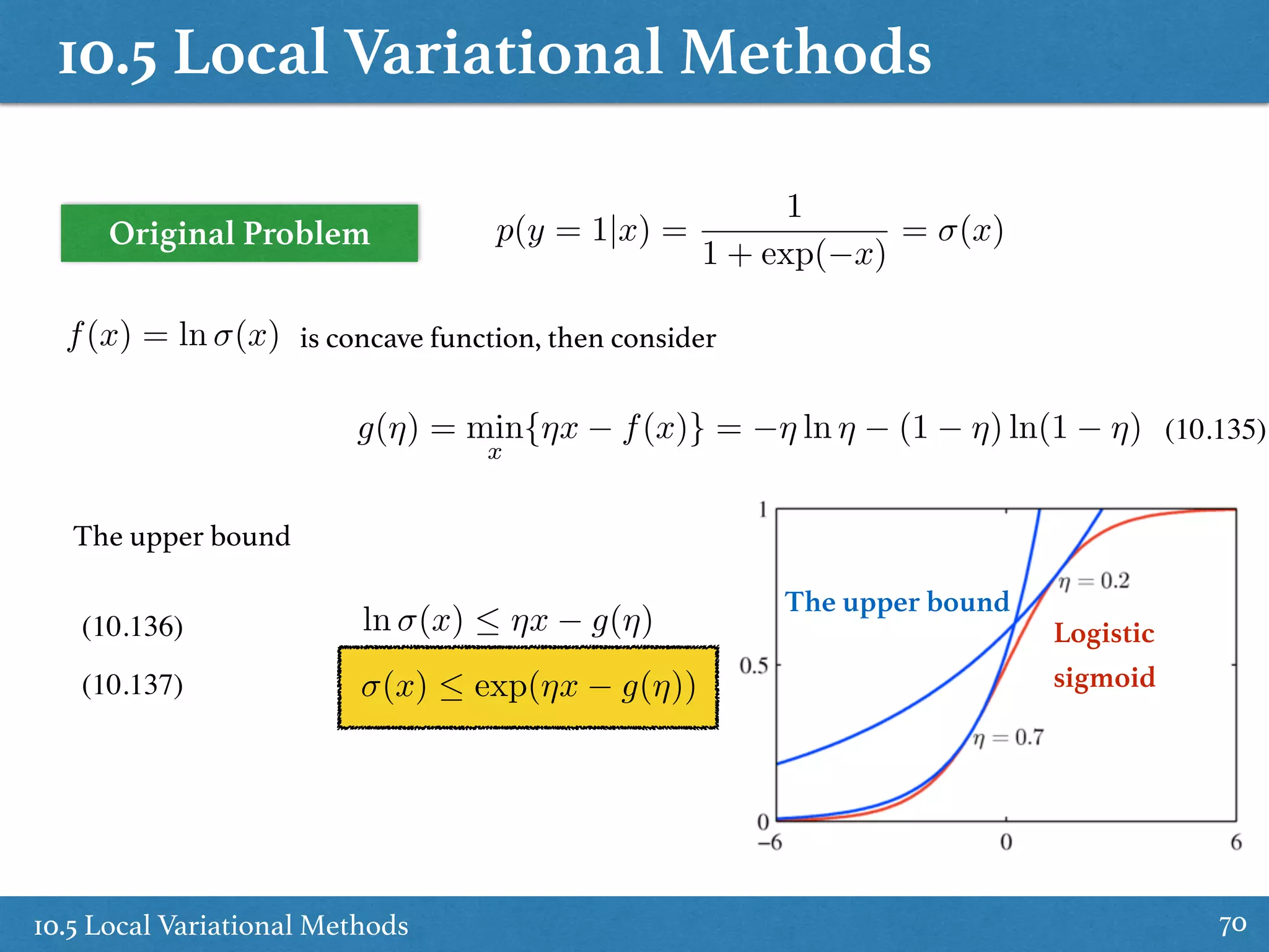
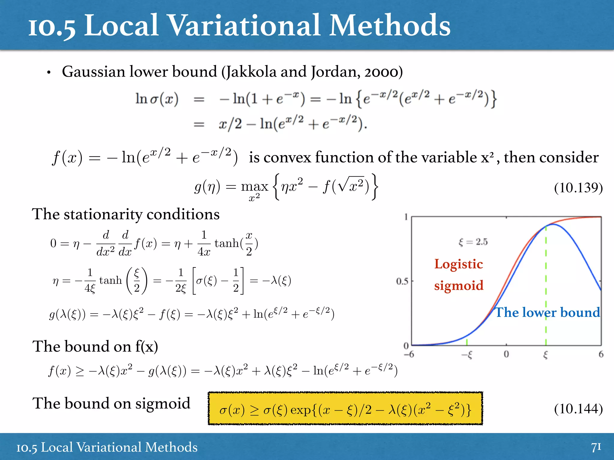
Introduction to local variational methods contrasting with global methods for posterior approximations.
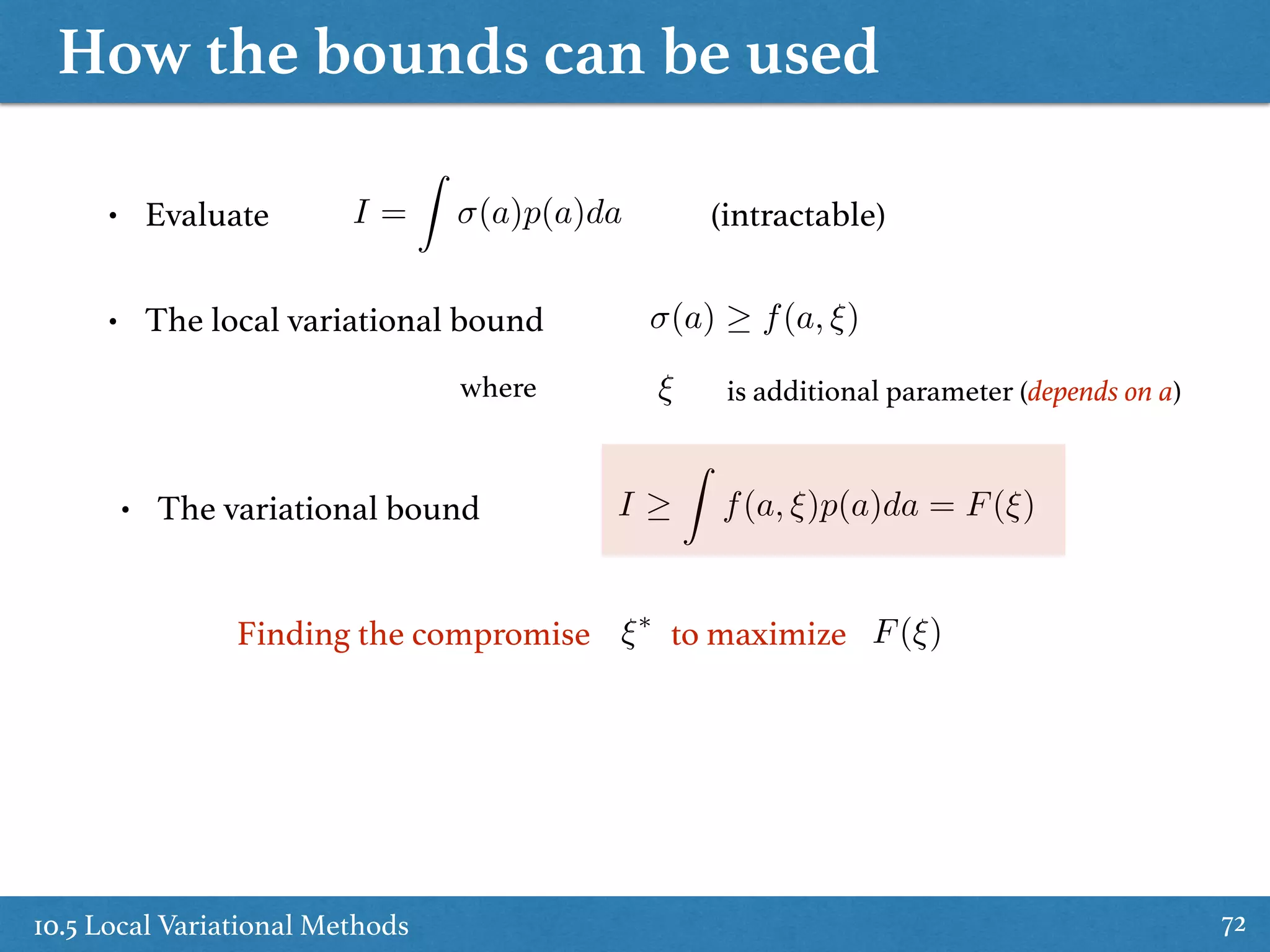
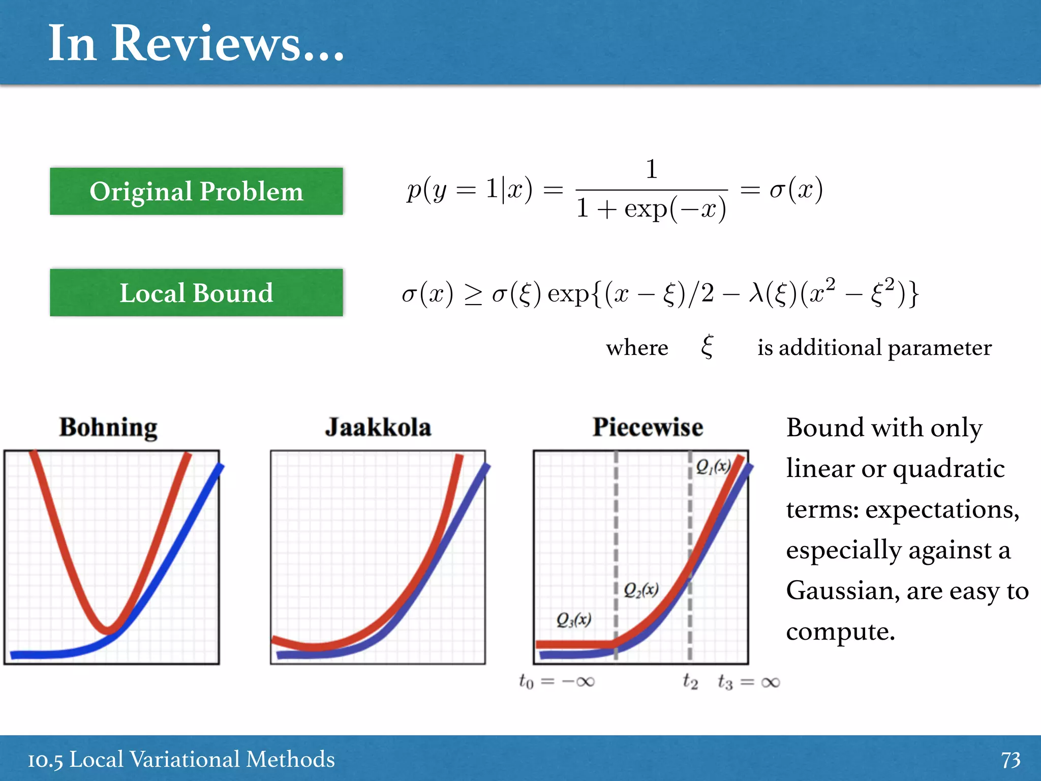
Practical applications and evaluations of local variational methods with respect to logistic models.
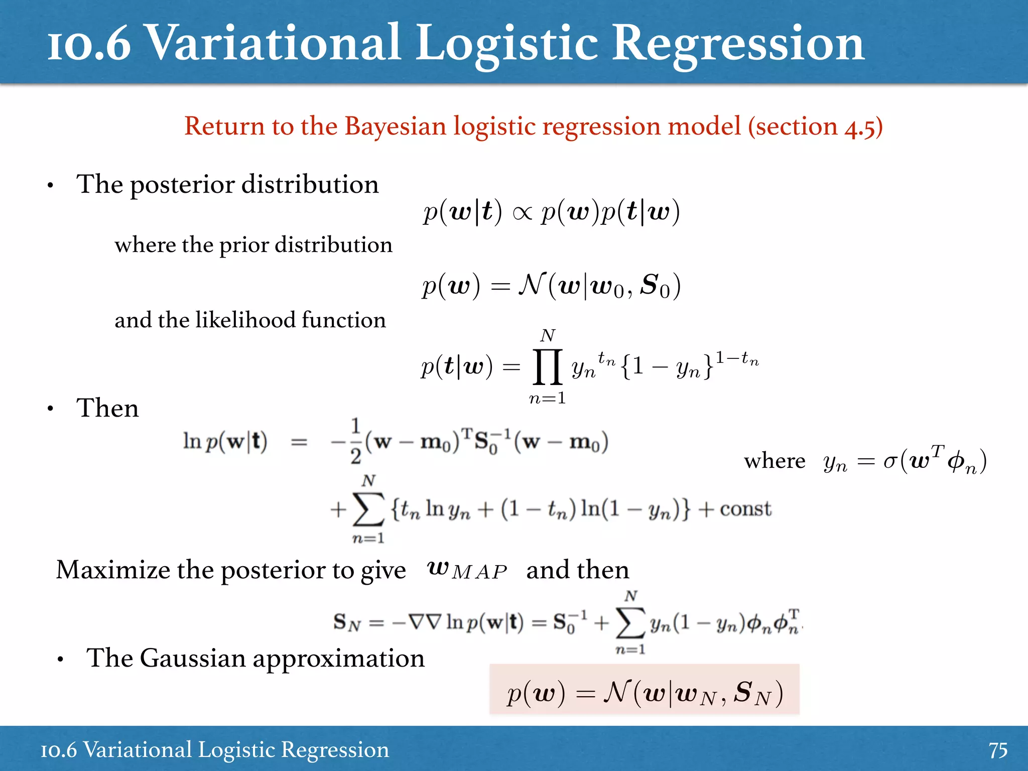
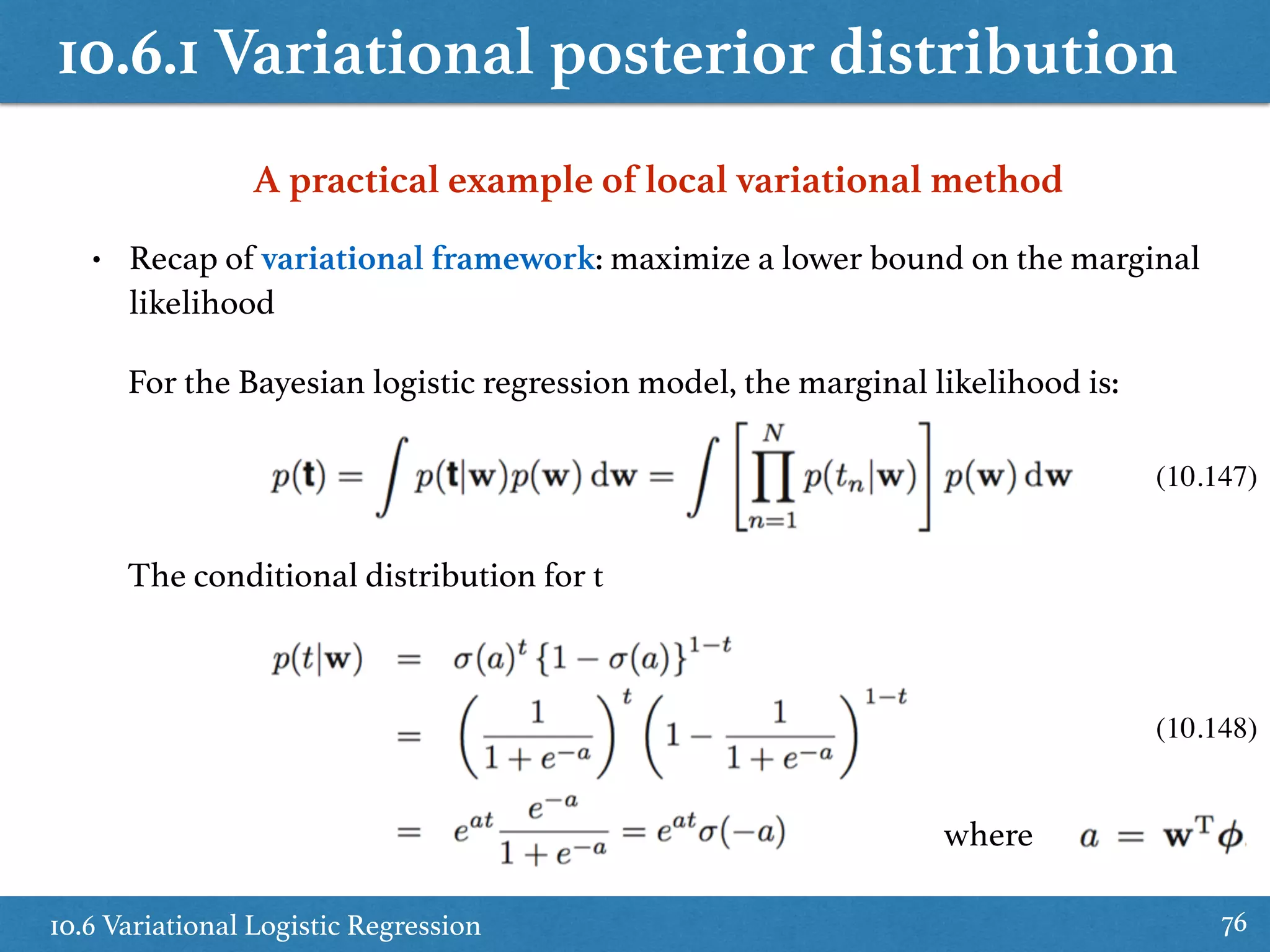
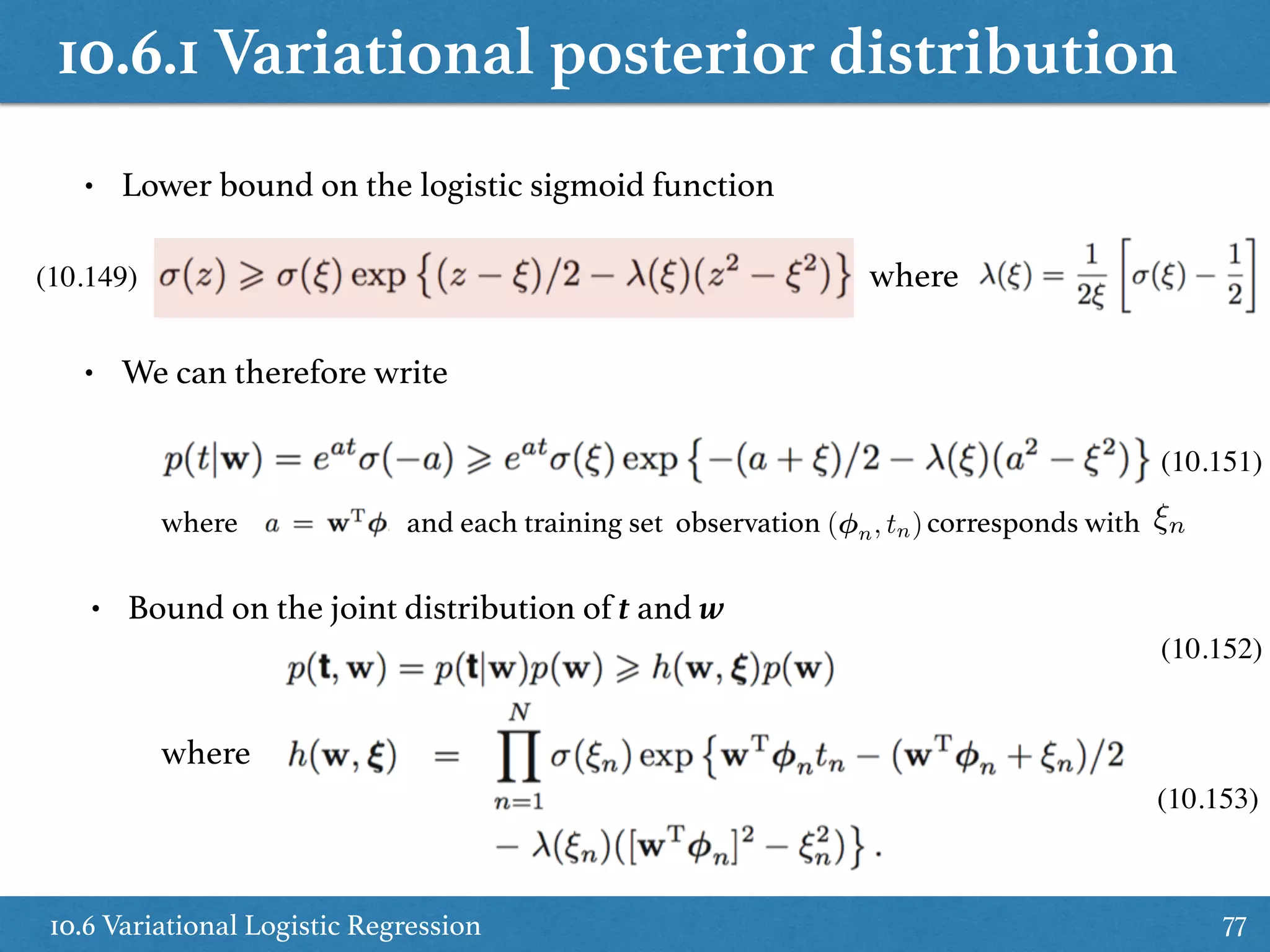
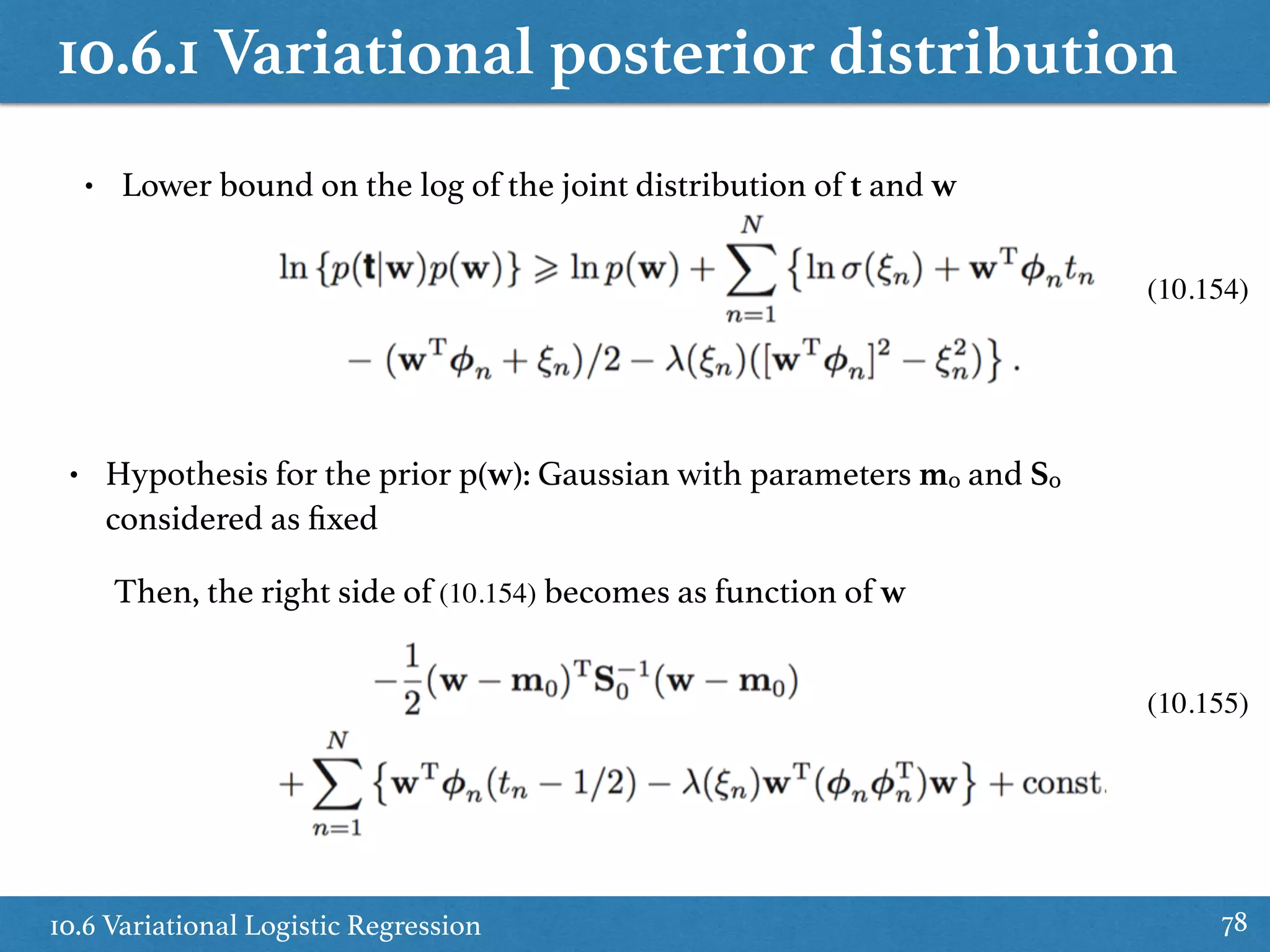
Revisits Bayesian logistic regression within the variational framework, detailing inference and parameter optimization.
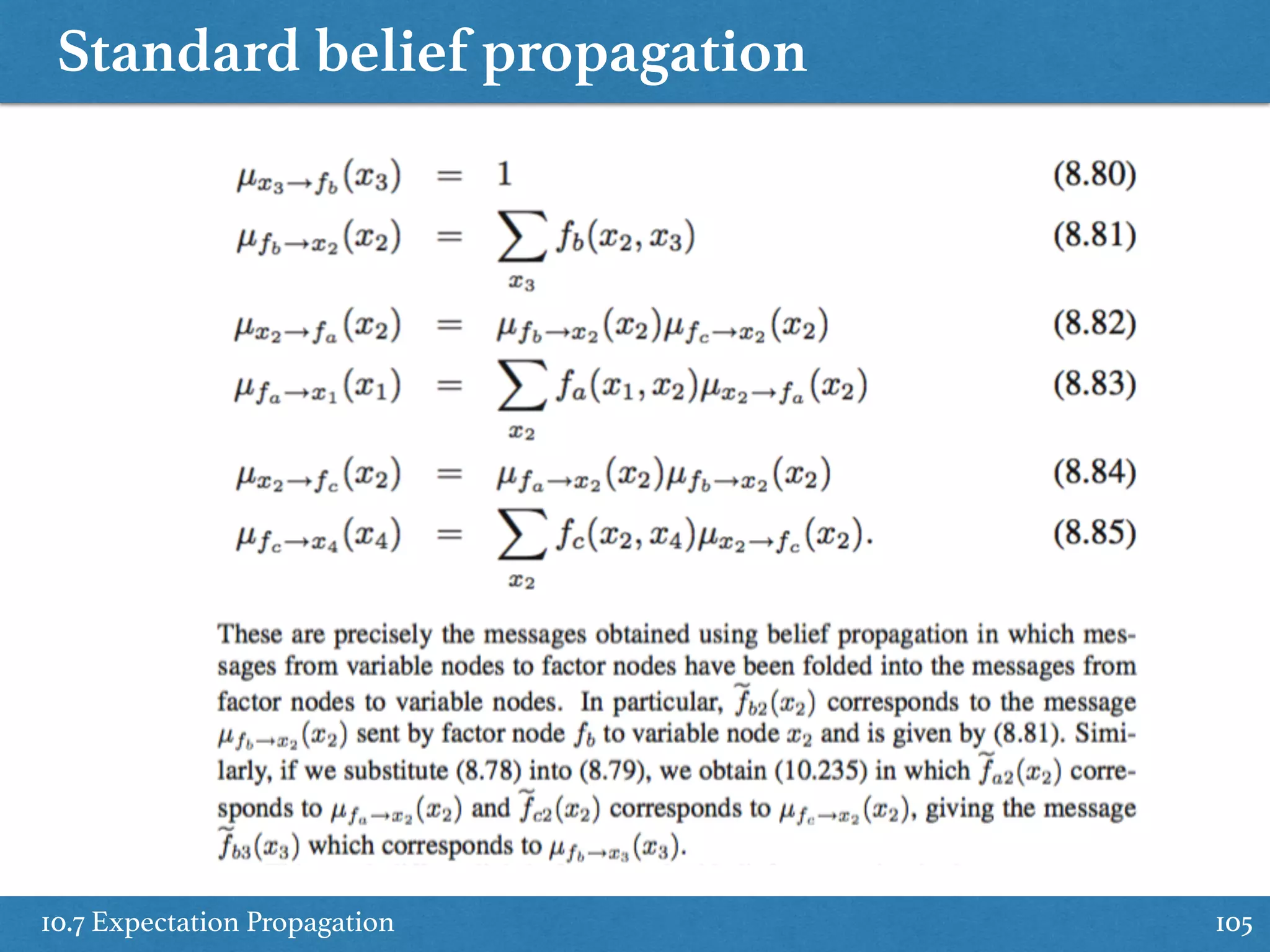
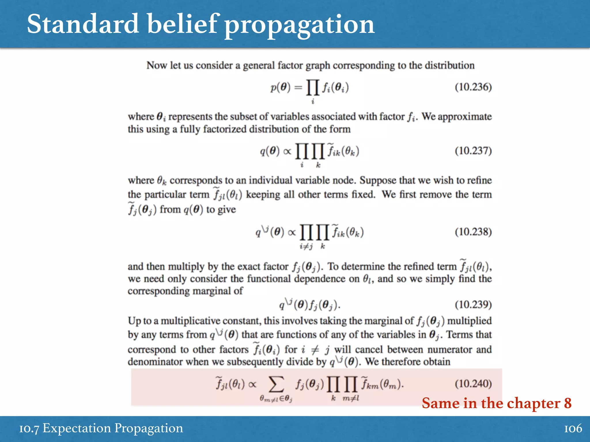
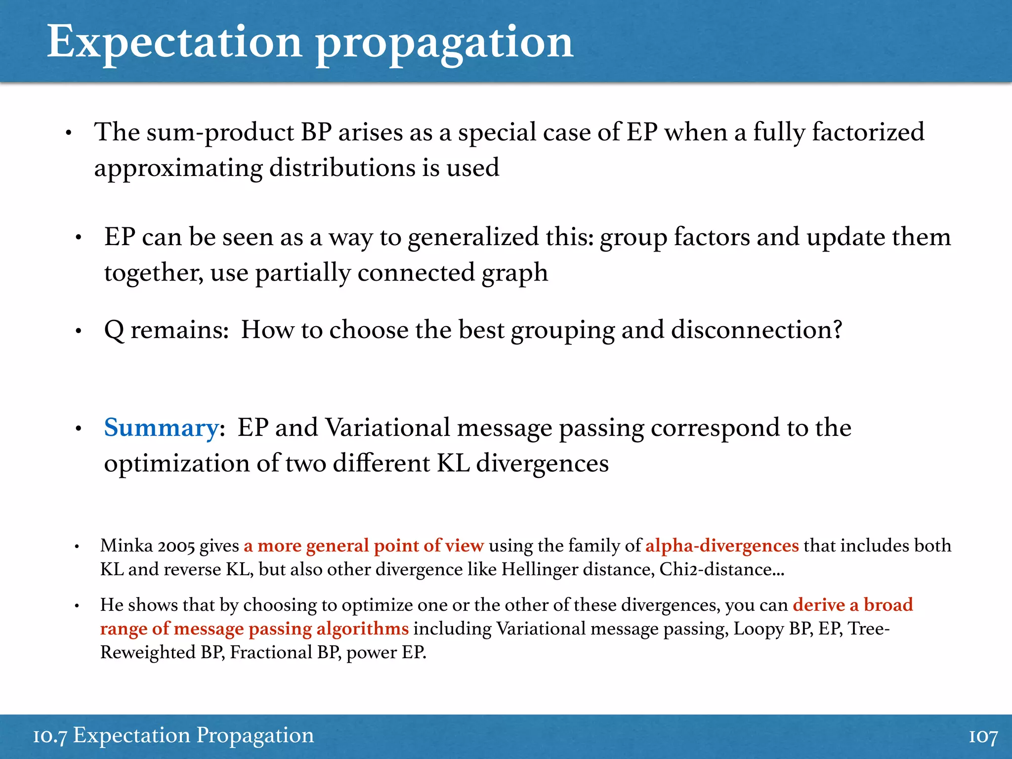
Explains expectation propagation methods as alternative deterministic approximate inference techniques.
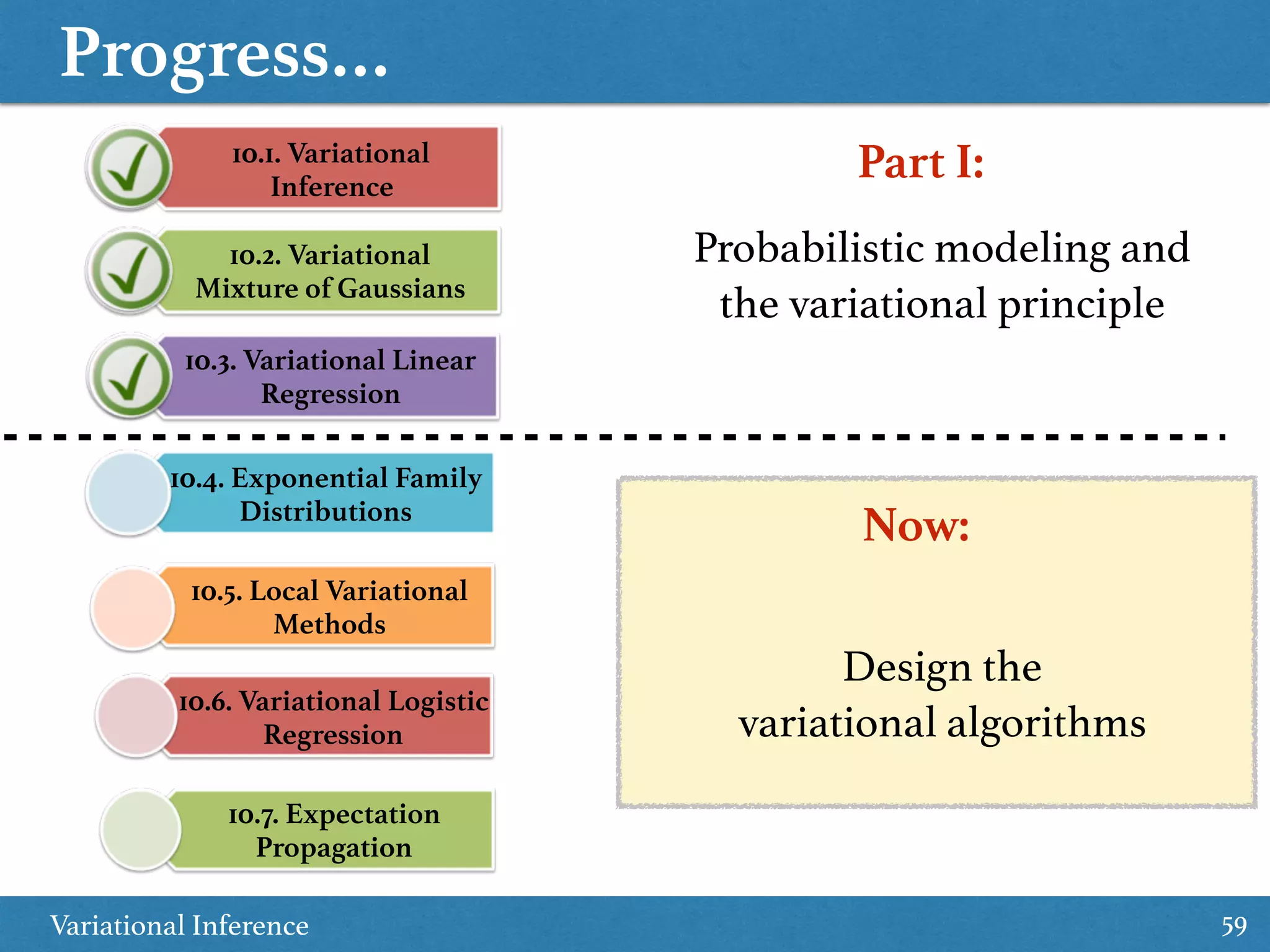
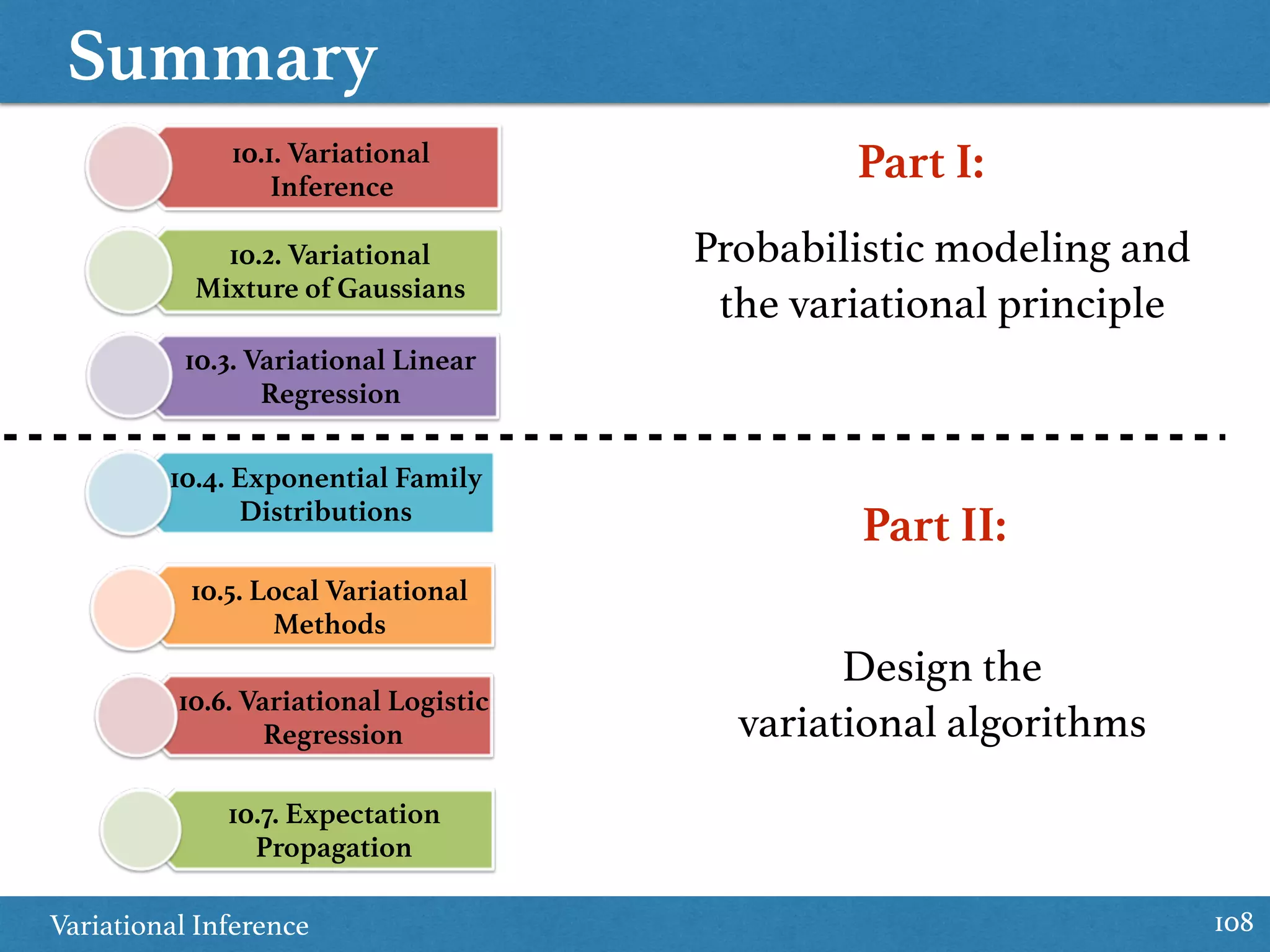
Summarizes key concepts in variational inference, emphasizing probabilistic modeling and algorithm design.

![[DL輪読会]Scalable Training of Inference Networks for Gaussian-Process Models](https://cdn.slidesharecdn.com/ss_thumbnails/mainslideshare1-190927025239-thumbnail.jpg?width=640&height=640&fit=bounds)


![[DL輪読会]Graph Convolutional Policy Network for Goal-Directed Molecular Graph G...](https://cdn.slidesharecdn.com/ss_thumbnails/graphconvolutionalpolicynetworkforgoal-directedmoleculargraphgeneration-181102004011-thumbnail.jpg?width=640&height=640&fit=bounds)


![Vibe Coding vs. Spec-Driven Development [Free Meetup]](https://cdn.slidesharecdn.com/ss_thumbnails/vibecodingvsspecdrivendevelopment-251209105622-43f455e7-thumbnail.jpg?width=640&height=640&fit=bounds)


