5--Test of hypothesis statistics (part_1).ppt

1
Function of Hypothesis Testing
Function of Hypothesis Testing
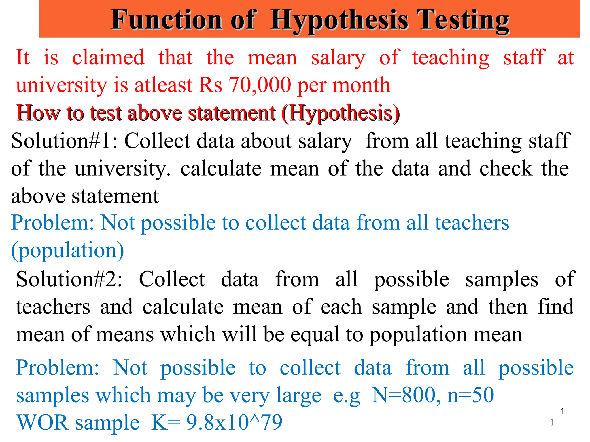
It is claimed that the mean salary of teaching staff at
university is atleast Rs 70,000 per month
How to test above statement (Hypothesis)
How to test above statement (Hypothesis)
Solution#1: Collect data about salary from all teaching staff
of the university. calculate mean of the data and check the
above statement
Problem: Not possible to collect data from all teachers
(population)
Solution#2: Collect data from all possible samples of
teachers and calculate mean of each sample and then find
mean of means which will be equal to population mean
Problem: Not possible to collect data from all possible
samples which may be very large e.g N=800, n=50
WOR sample K= 9.8x10^79 1

2
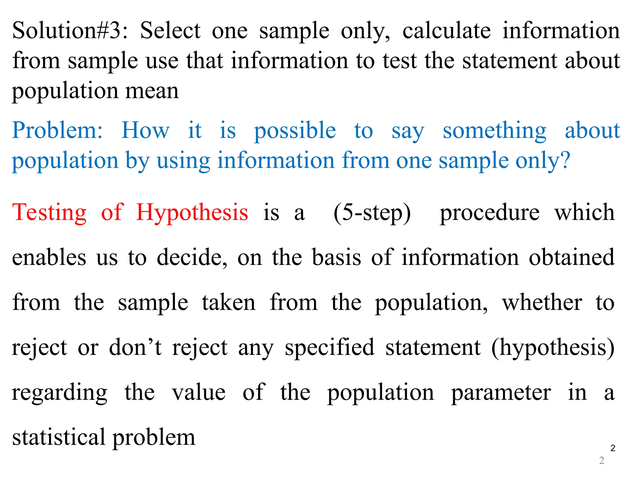
Solution#3: Select one sample only, calculate information
from sample use that information to test the statement about
population mean
Problem: How it is possible to say something about
population by using information from one sample only?
Testing of Hypothesis is a (5-step) procedure which
enables us to decide, on the basis of information obtained
from the sample taken from the population, whether to
reject or don’t reject any specified statement (hypothesis)
regarding the value of the population parameter in a
statistical problem
2

Sampling
Population
Sample
Subset
The process of selecting a sample (representative
part) from a population is called SAMPLING
3

4
4
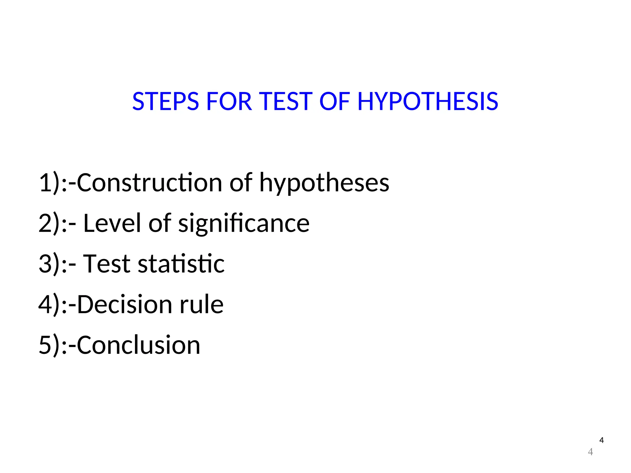
STEPS FOR TEST OF HYPOTHESIS
1):-Construction of hypotheses
2):- Level of significance
3):- Test statistic
4):-Decision rule
5):-Conclusion
4

5
1/5
1/5 Construction of hypotheses
Construction of hypotheses
[
[Null and Alternative Hypotheses]
Null and Alternative Hypotheses]
The null hypothesis, denoted H0, is any hypothesis which is
to be tested for possible rejection or nullification under the
assumption that it is true. The null hypothesis always
contains some form of an equality sign.
The alternative hypothesis, denoted H1, The complement of
the null hypothesis is called the alternative hypothesis. It is
denoted by H1. The alternative hypothesis never contains
the sign of equality and is always in an inequality form.
A Statistical Hypothesis is an assumption made about the
population parameter which may or may not be true.
5

6
1/5
[One sided and two sided hypothesis]
[One sided and two sided hypothesis]
One-Sided, Less Than (Left Tail)
H0:   50 H1:  < 50
One-Sided, Greater Than ( Right Tail)
H0:   50 H1:  > 50
Two-Sided, Not Equal To
H0:  = 50 H1:   50
6
Test the hypothesis that population mean is more than 50:  > 50
Test the hypothesis that population mean is atleast 50:   50

7
1/5
[
[Null and Alternative Hypotheses]
Null and Alternative Hypotheses]
Example:
A major west coast city provides one of the most
comprehensive emergency medical services in the
world. The service goal is to respond to medical
emergencies with a mean time of 12 minutes or less.
The director of medical services wants to
formulate a hypothesis test that could use a sample
of emergency response times to determine whether
or not the service goal of 12 minutes is being
achieved. 7

• Null and Alternative Hypotheses
Hypotheses Conclusion and Action
H0:  The emergency service is meeting
the response goal; no follow-up
action is necessary.
H1: The emergency service is not
meeting the response goal;
appropriate follow-up action is
necessary.
Where:  = mean response time for the population
of medical emergency requests.
1/5
[Construction of Hypotheses]
[Construction of Hypotheses]
8

9
2/5 Level of significance
[Type I and Type II errors]
Whenever sample evidence is used to draw a conclusion about population, there are
risks of making wrong decision because of sampling.
Such errors in making the incorrect conclusion are called Inferential Errors,
because they entail drawing an incorrect inference from the sample about the value
of the population parameter.
On the basis of sample information, we may reject a true statement about
population or don’t reject a false statement
Type I error = Reject H0 when in fact H0 true
Type II error = Don’t Reject H0 when in fact H0 is false
9

10
• Significance Level
Probability of committing a Type-I error is called the level of
significance, denoted by α .
The level of significance is also called the size of test.
By α =5% we mean that there are 5 chances in 100 of incorrectly
rejecting a true null hypothesis.
To put it in another way we say that we are 95% confident in
making the correct decision.
• Level of Confidence
The probability of not committing a Type-I error, (1- α ), is called
the level of confidence, or confidence co-efficient.
10

11
3/5 Test Statistic
3/5 Test Statistic
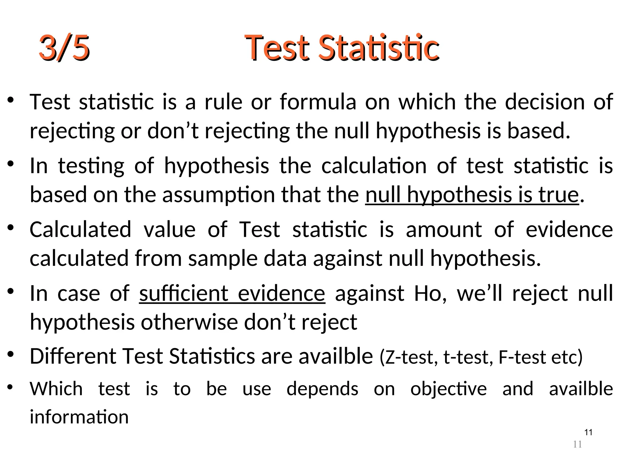
• Test statistic is a rule or formula on which the decision of
rejecting or don’t rejecting the null hypothesis is based.
• In testing of hypothesis the calculation of test statistic is
based on the assumption that the null hypothesis is true.
• Calculated value of Test statistic is amount of evidence
calculated from sample data against null hypothesis.
• In case of sufficient evidence against Ho, we’ll reject null
hypothesis otherwise don’t reject
• Different Test Statistics are availble (Z-test, t-test, F-test etc)
• Which test is to be use depends on objective and availble
information
11

12
4/5 Decision Rule
4/5 Decision Rule
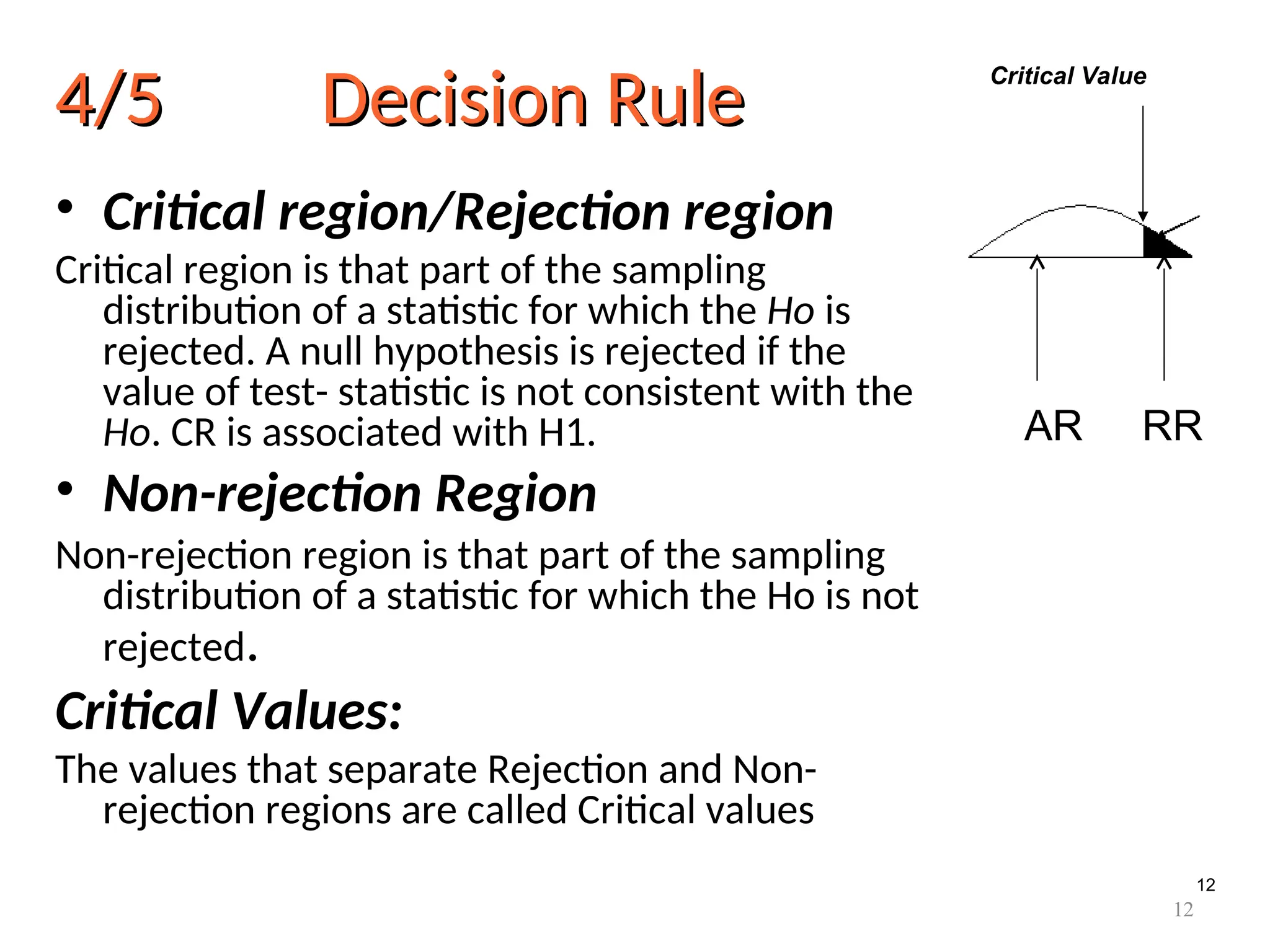
• Critical region/Rejection region
Critical region is that part of the sampling
distribution of a statistic for which the Ho is
rejected. A null hypothesis is rejected if the
value of test- statistic is not consistent with the
Ho. CR is associated with H1.
• Non-rejection Region
Non-rejection region is that part of the sampling
distribution of a statistic for which the Ho is not
rejected.
Critical Values:
The values that separate Rejection and Non-
rejection regions are called Critical values
AR RR
Critical Value
12

13
5/5 Conclusion
5/5 Conclusion
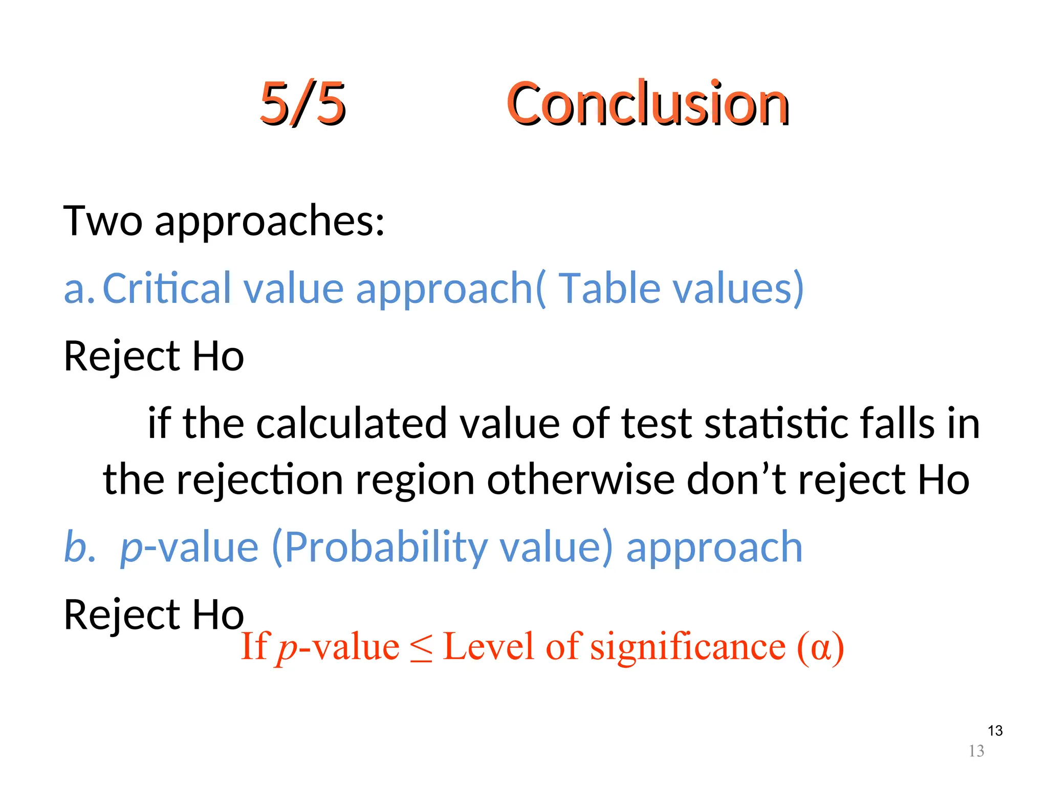
Two approaches:
a.Critical value approach( Table values)
Reject Ho
if the calculated value of test statistic falls in
the rejection region otherwise don’t reject Ho
b. p-value (Probability value) approach
Reject Ho
If p-value ≤ Level of significance (α)
13

14
2
X
Z
n




 
 
 
 
2
X
Z
n
S



 
 
 
 
Yes
Yes
NO
NO
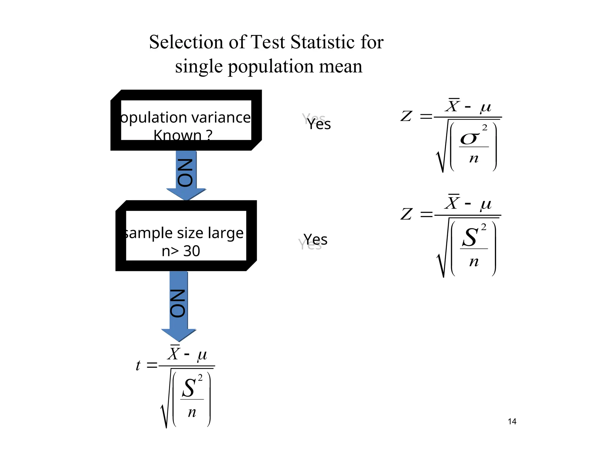
Population variance
Known ?
sample size large
n> 30
2
X
t
n
S



 
 
 
 
Selection of Test Statistic for
single population mean

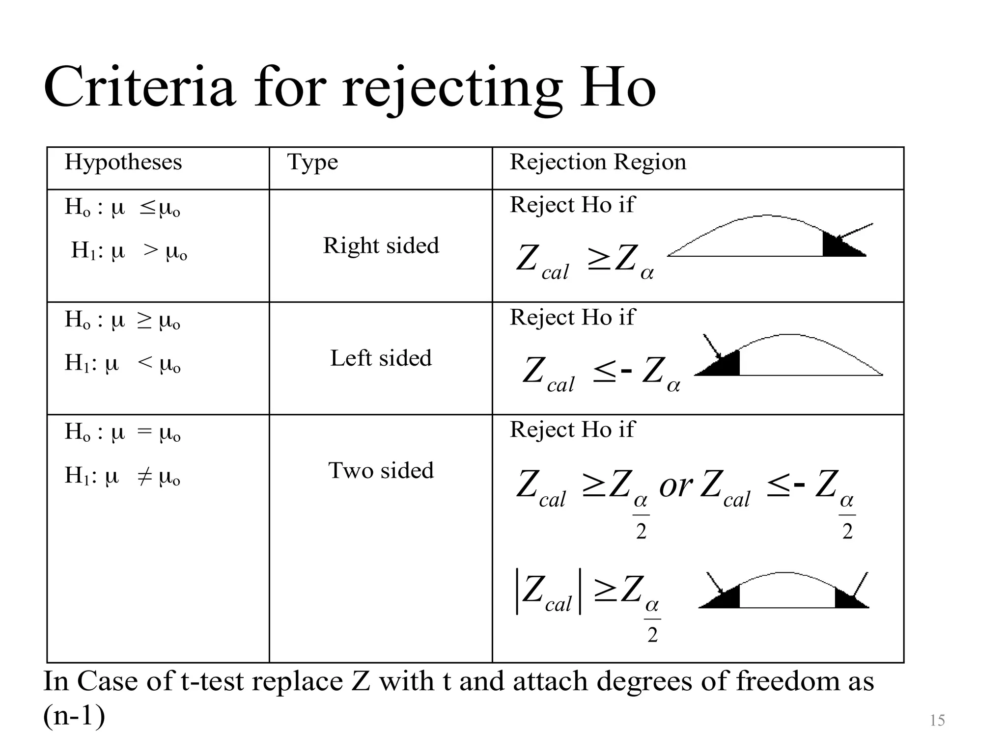
Criteria for rejecting Ho
Hypotheses Type Rejection Region
Ho :  o
H1:  > o Right sided
Reject Ho if

Z
Zcal 
Ho :  ≥ o
H1:  < o Left sided
Reject Ho if

Z
Zcal 

Ho :  = o
H1:  ≠ o Two sided
Reject Ho if
2 2
cal cal
Z Z or Z Z
 
 
2
cal
Z Z

In Case of t-test replace Z with t and attach degrees of freedom as
(n-1) 15

16
16
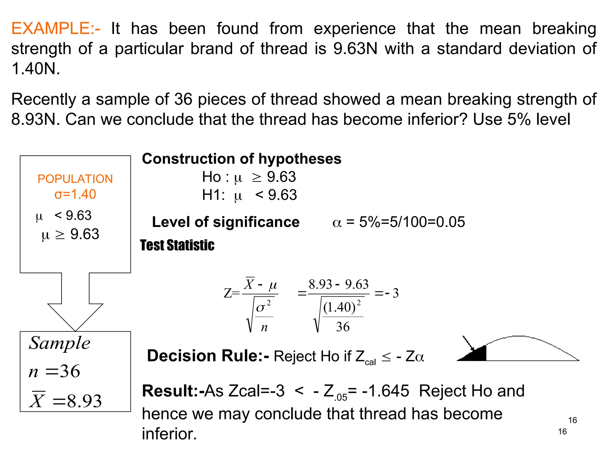
EXAMPLE:- It has been found from experience that the mean breaking
strength of a particular brand of thread is 9.63N with a standard deviation of
1.40N.
Recently a sample of 36 pieces of thread showed a mean breaking strength of
8.93N. Can we conclude that the thread has become inferior? Use 5% level
POPULATION
σ=1.40
Ho :   9.63
H1:  < 9.63
Level of significance  = 5%=5/100=0.05
Decision Rule:- Reject Ho if Zcal  - Z
Result:-As Zcal=-3 < - Z.05= -1.645 Reject Ho and
hence we may conclude that thread has become
inferior.
 < 9.63
  9.63
Test Statistic
Z=
n
X
2



3
36
)
40
.
1
(
63
.
9
93
.
8
2




93
.
8
36


X
n
Sample

17
17
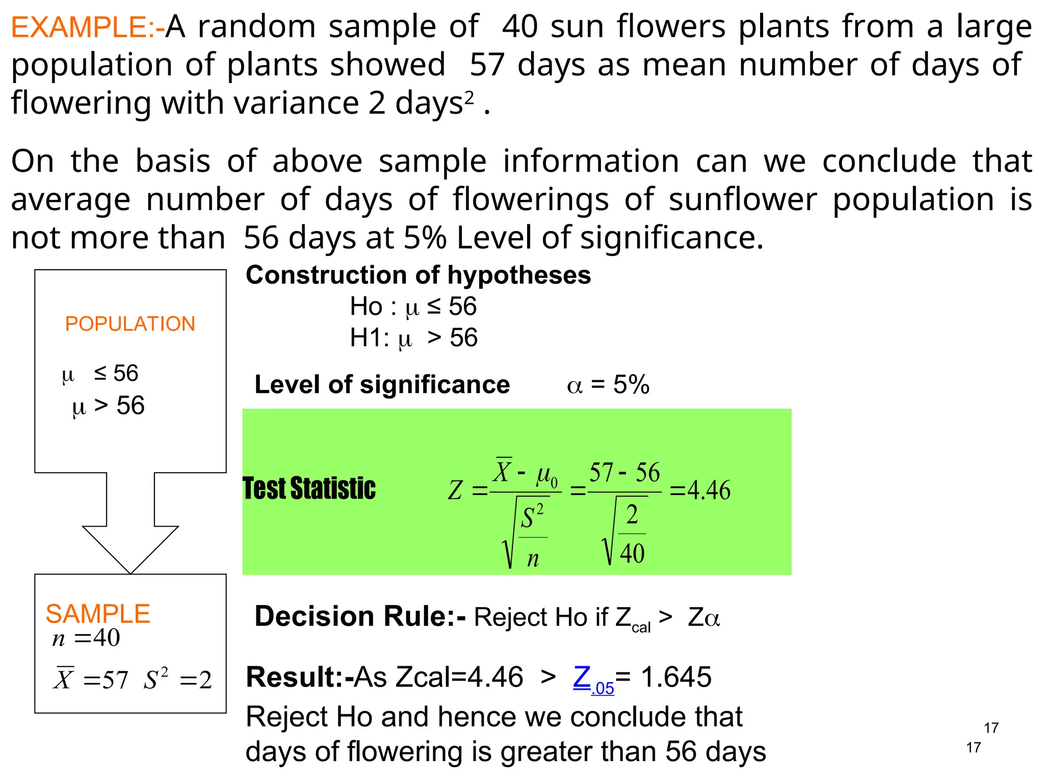
EXAMPLE:-A random sample of 40 sun flowers plants from a large
population of plants showed 57 days as mean number of days of
flowering with variance 2 days2
.
On the basis of above sample information can we conclude that
average number of days of flowerings of sunflower population is
not more than 56 days at 5% Level of significance.
POPULATION
SAMPLE
Ho :  ≤ 56
H1:  > 56
Level of significance  = 5%
Decision Rule:- Reject Ho if Zcal > Z
Result:-As Zcal=4.46 > Z.05= 1.645
Reject Ho and hence we conclude that
days of flowering is greater than 56 days
 ≤ 56
 > 56
Test Statistic 46
.
4
40
2
56
57
2
0





n
S
X
Z

2
57
40
2



S
X
n

18
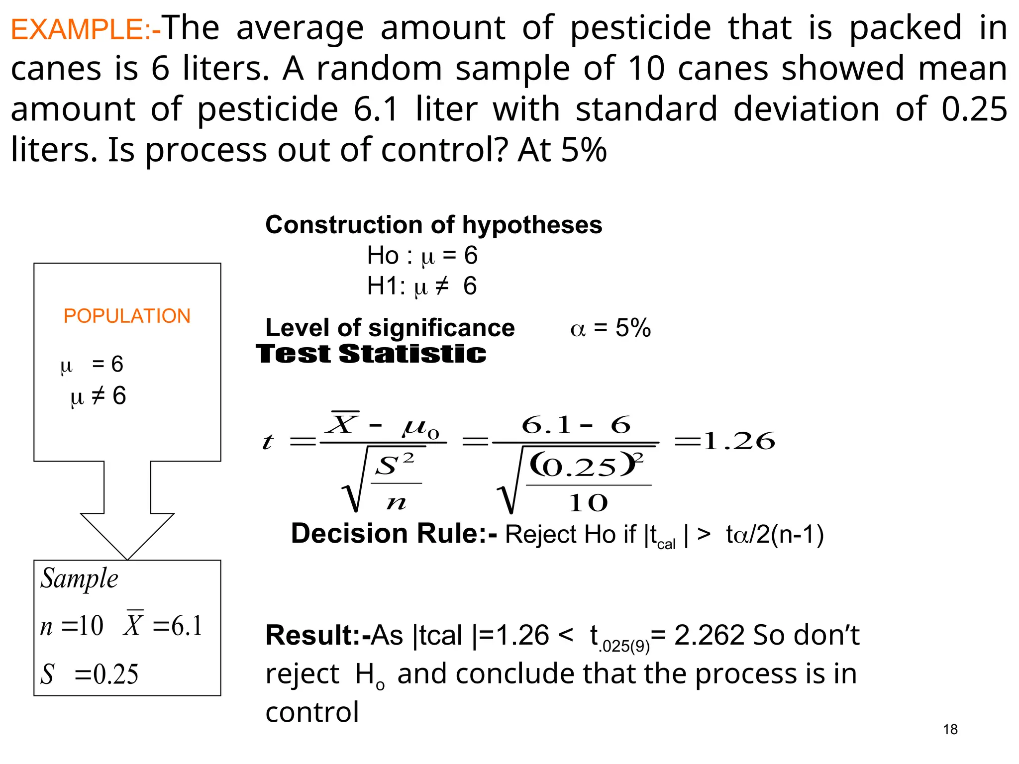
EXAMPLE:-The average amount of pesticide that is packed in
canes is 6 liters. A random sample of 10 canes showed mean
amount of pesticide 6.1 liter with standard deviation of 0.25
liters. Is process out of control? At 5%
POPULATION
Ho :  = 6
H1:  ≠ 6
Level of significance  = 5%
Decision Rule:- Reject Ho if |tcal | > t/2(n-1)
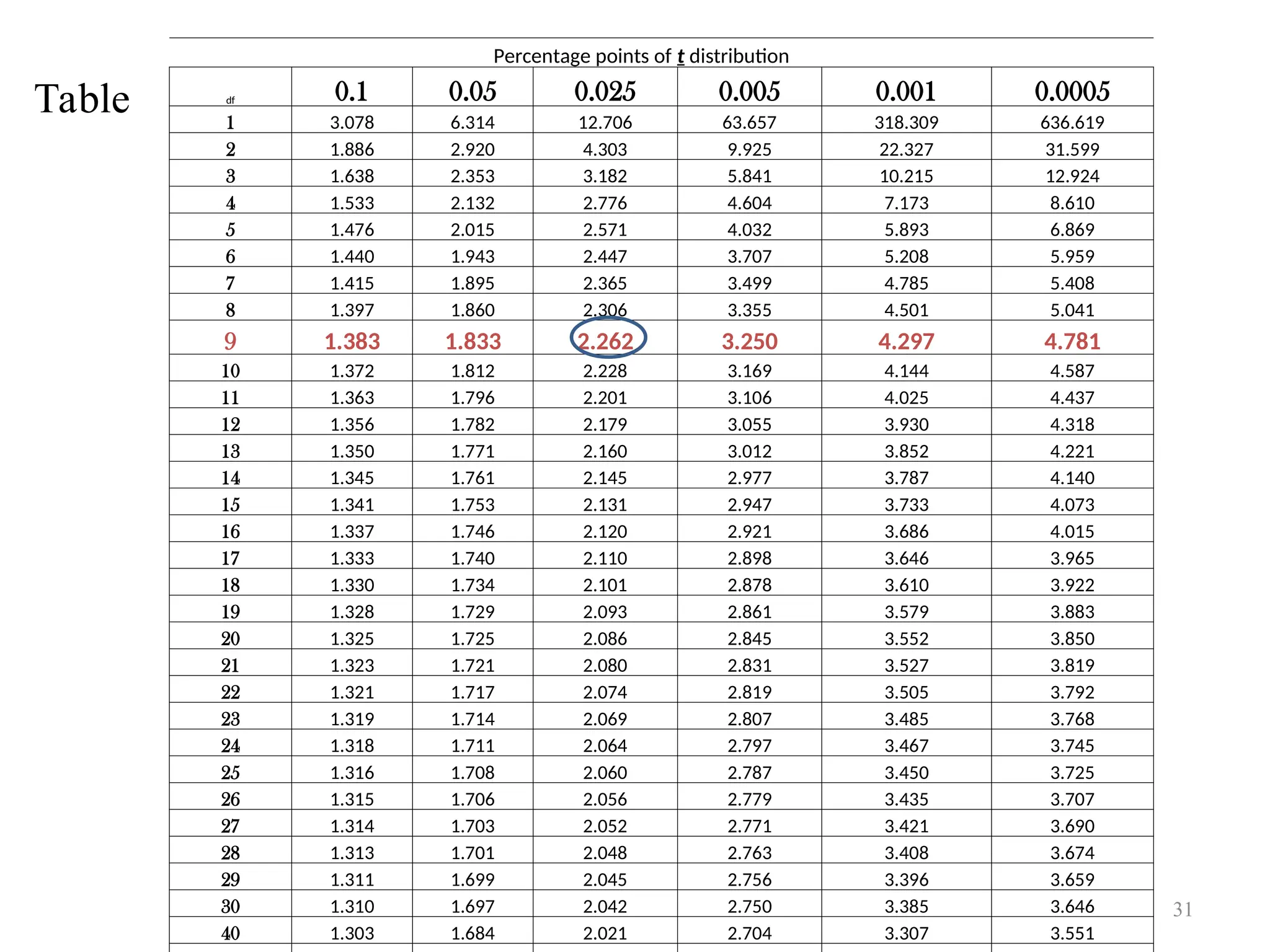
Result:-As |tcal |=1.26 < t.025(9)= 2.262 So don’t
reject Ho and conclude that the process is in
control
 = 6
 ≠ 6
Test Statistic
 
26
.
1
10
25
.
0
6
1
.
6
2
2
0





n
S
X
t

25
.
0
1
.
6
10



S
X
n
Sample

19
19
POPULATION PARAMETER ?
Point Estimate
(Single value)
Interval Estimate
(Range of Values)

20
20
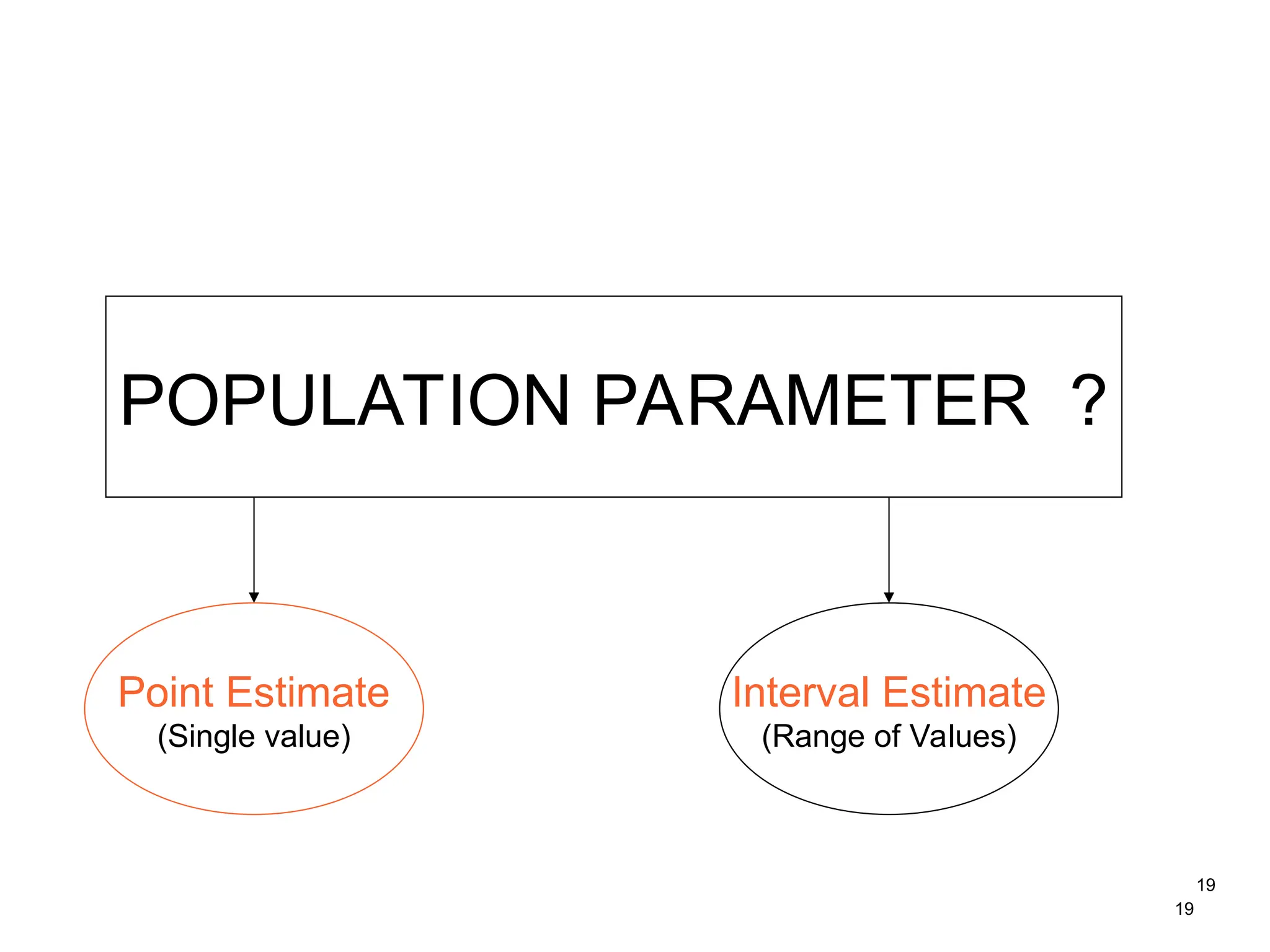
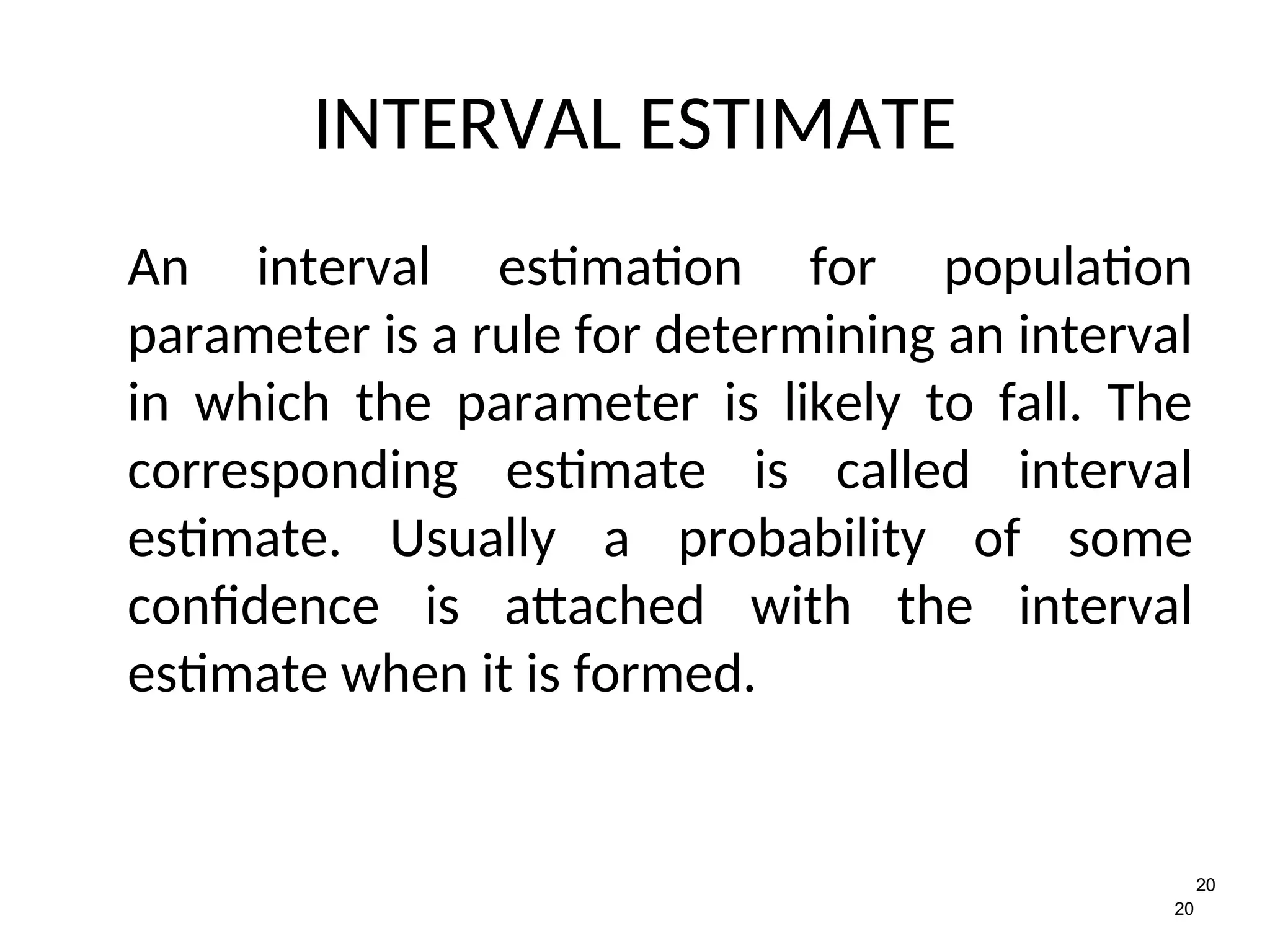
INTERVAL ESTIMATE
An interval estimation for population
parameter is a rule for determining an interval
in which the parameter is likely to fall. The
corresponding estimate is called interval
estimate. Usually a probability of some
confidence is attached with the interval
estimate when it is formed.

21
21
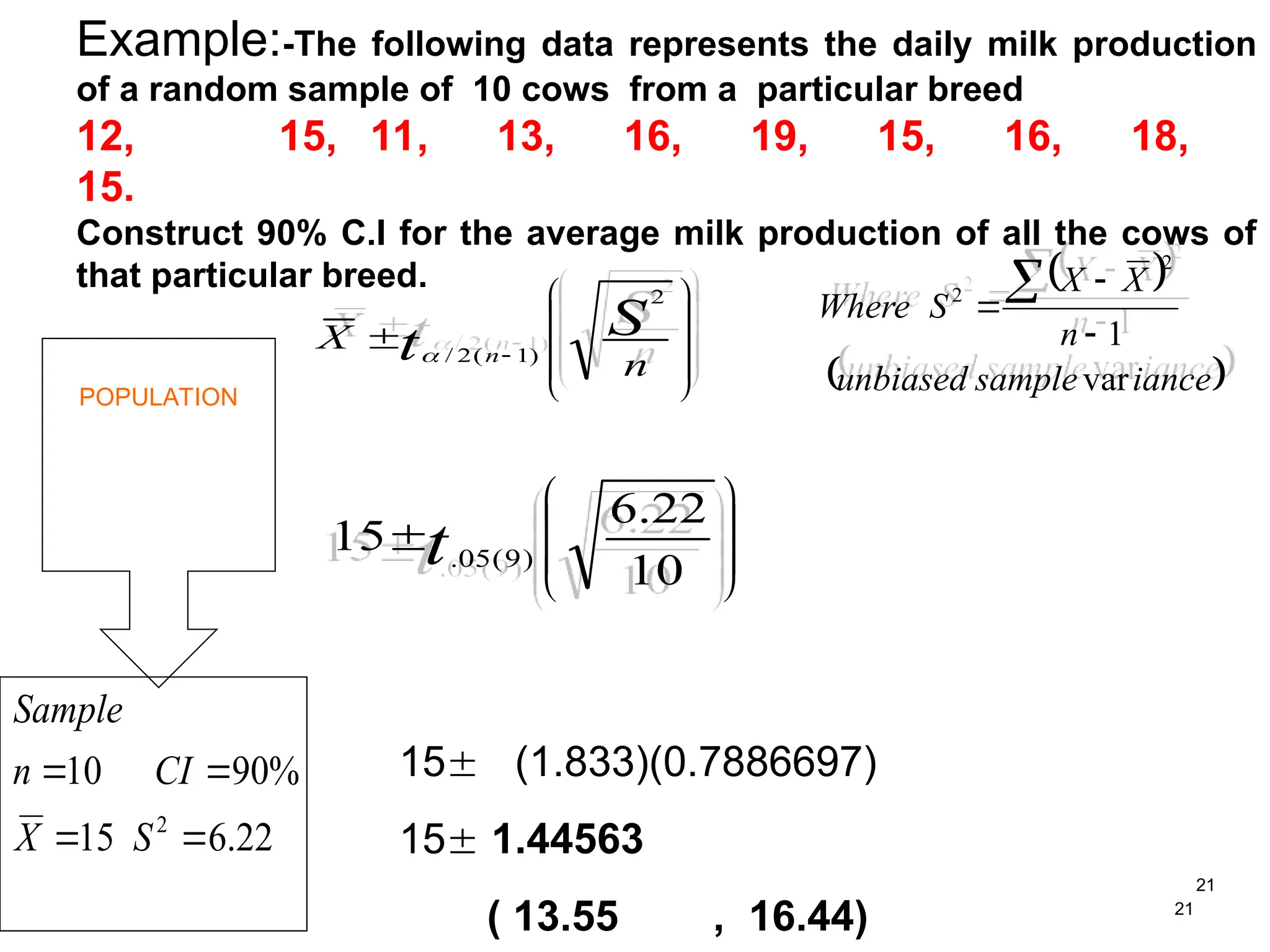
Example:-The following data represents the daily milk production
of a random sample of 10 cows from a particular breed
12, 15, 11, 13, 16, 19, 15, 16, 18,
15.
Construct 90% C.I for the average milk production of all the cows of
that particular breed.
POPULATION










 
n
X S
t n
2
)
1
(
2
/










10
22
.
6
15 )
9
(
05
.
t
22
.
6
15
%
90
10
2




S
X
CI
n
Sample
 
 
iance
sample
unbiased
n
X
X
S
Where
var
1
2
2




15 (1.833)(0.7886697)
15 1.44563
( 13.55 , 16.44)

22
   











2
1
1
1
2
2
1
2
1
n
n
X
X
t
Sp


   













2
1
2
2
2
1
2
1
2
1
n
n
X
X
Z




   













2
1
2
2
2
1
2
1
2
1
n
n
X
X
Z
S
S


Yes
Yes
NO
NO
Population variances
are Known
Both samples
are large
(n1 & n2 )> 30
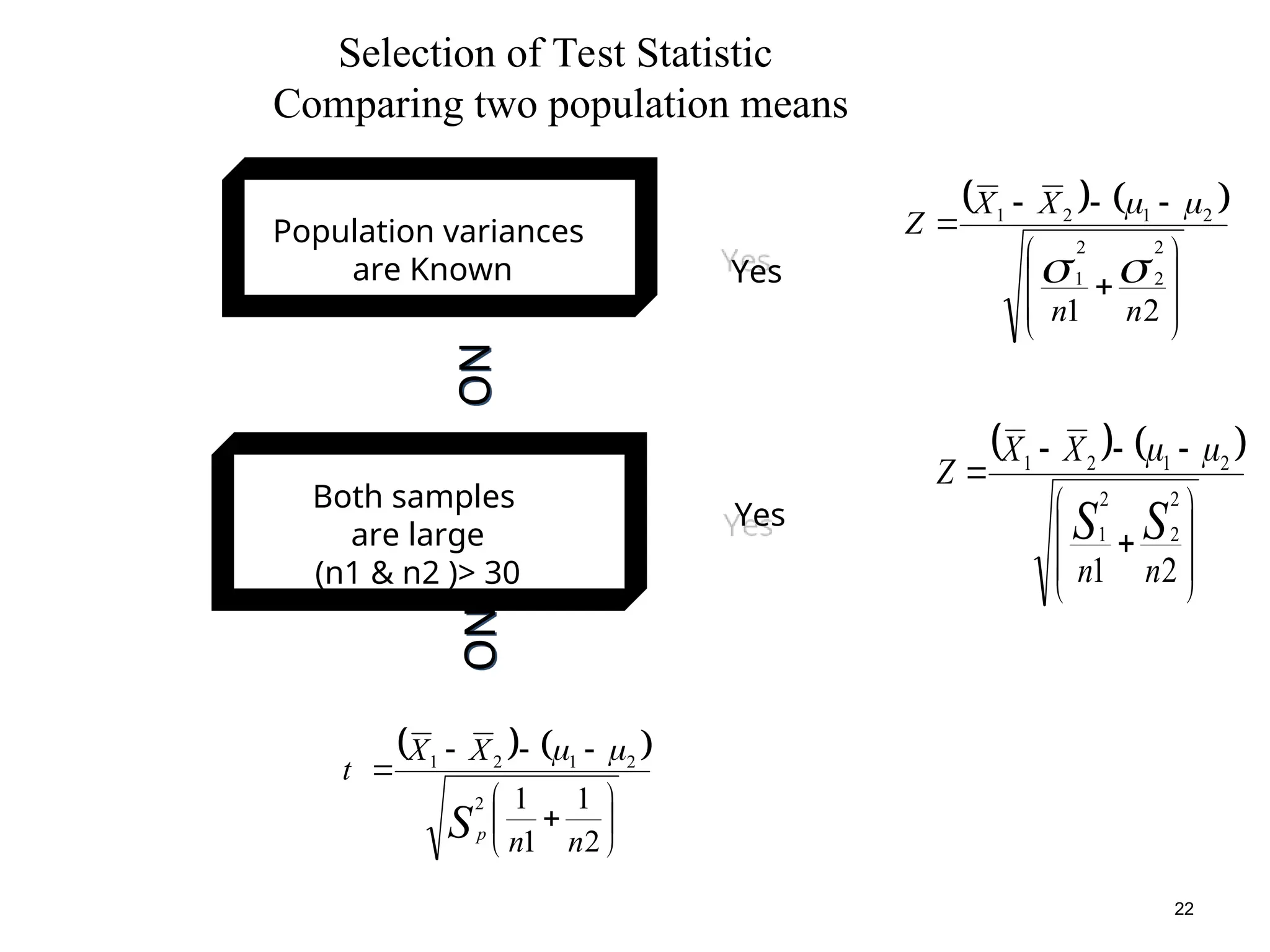
Selection of Test Statistic
Comparing two population means

23
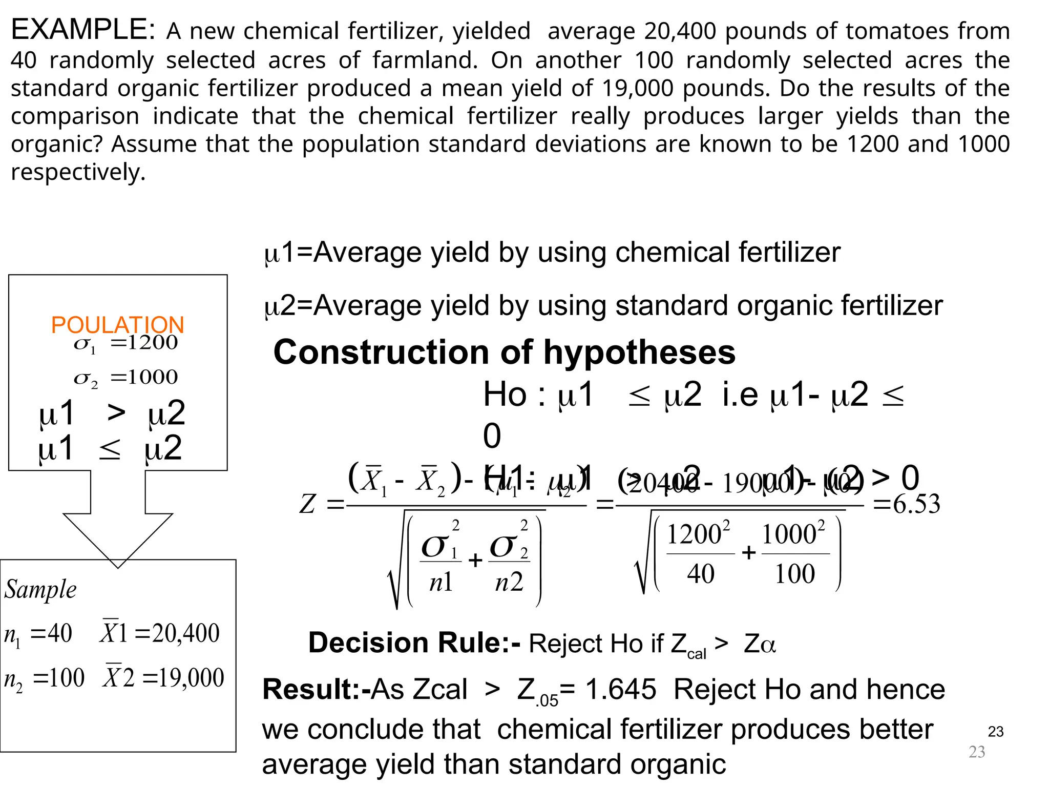
EXAMPLE: A new chemical fertilizer, yielded average 20,400 pounds of tomatoes from
40 randomly selected acres of farmland. On another 100 randomly selected acres the
standard organic fertilizer produced a mean yield of 19,000 pounds. Do the results of the
comparison indicate that the chemical fertilizer really produces larger yields than the
organic? Assume that the population standard deviations are known to be 1200 and 1000
respectively.
POULATION
Ho : 1  2 i.e 1- 2 
0
H1: 1 > 2 1- 2 > 0
1 > 2
1  2
1=Average yield by using chemical fertilizer
2=Average yield by using standard organic fertilizer
000
,
19
2
100
400
,
20
1
40
2
1




X
n
X
n
Sample
1000
1200
2
1




       
1 2 1 2
2 2 2 2
1 2
20400 19000 0
6.53
1200 1000
40 100
1 2
X X
Z
n n
 
 
    
  
   

   

   
 
Decision Rule:- Reject Ho if Zcal > Z
Result:-As Zcal > Z.05= 1.645 Reject Ho and hence
we conclude that chemical fertilizer produces better
average yield than standard organic
23

24
24
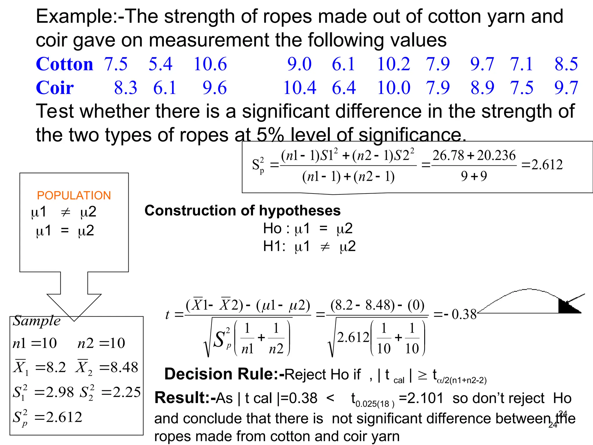
Example:-The strength of ropes made out of cotton yarn and
coir gave on measurement the following values
Cotton 7.5 5.4 10.6 9.0 6.1 10.2 7.9 9.7 7.1 8.5
Coir 8.3 6.1 9.6 10.4 6.4 10.0 7.9 8.9 7.5 9.7
Test whether there is a significant difference in the strength of
the two types of ropes at 5% level of significance.
POPULATION
Ho : 1 = 2
H1: 1  2
Decision Rule:-Reject Ho if , | t cal |  t/2(n1+n2-2)
Result:-As | t cal |=0.38 < t0.025(18 ) =2.101 so don’t reject Ho
and conclude that there is not significant difference between the
ropes made from cotton and coir yarn
1  2
1 = 2
38
.
0
10
1
10
1
612
.
2
)
0
(
)
48
.
8
2
.
8
(
2
1
1
1
)
2
1
(
)
2
1
(
2























n
n
X
X
t
Sp


612
.
2
9
9
236
.
20
78
.
26
)
1
2
(
)
1
1
(
2
)
1
2
(
1
)
1
1
(
S
2
2
2
p 










n
n
S
n
S
n
612
.
2
25
.
2
98
.
2
48
.
8
2
.
8
10
2
10
1
2
2
2
2
1
2
1







p
S
S
S
X
X
n
n
Sample

25
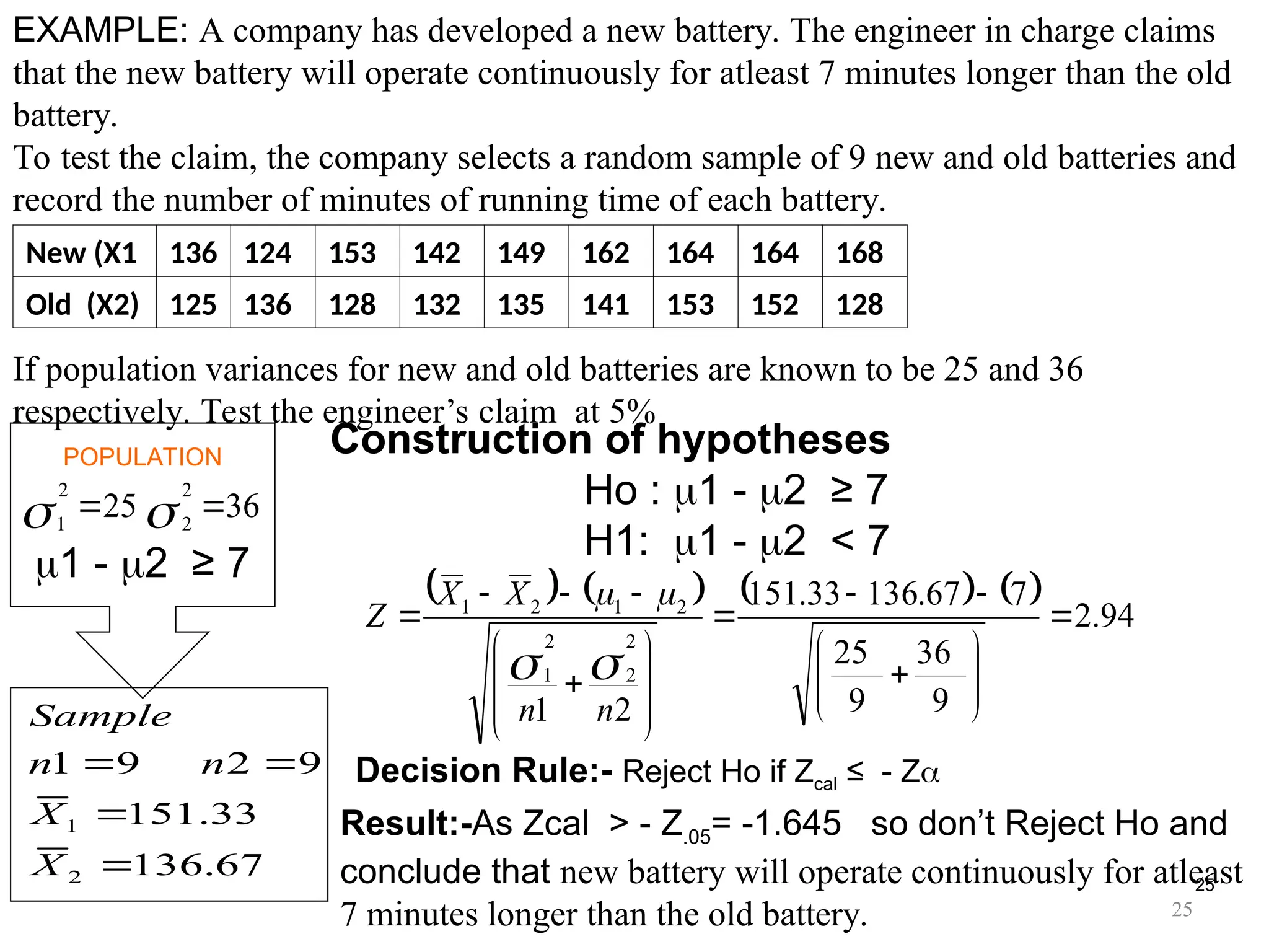
EXAMPLE: A company has developed a new battery. The engineer in charge claims
that the new battery will operate continuously for atleast 7 minutes longer than the old
battery.
To test the claim, the company selects a random sample of 9 new and old batteries and
record the number of minutes of running time of each battery.
If population variances for new and old batteries are known to be 25 and 36
respectively. Test the engineer’s claim at 5%
POPULATION Construction of hypotheses
Ho : 1 - 2 ≥ 7
H1: 1 - 2 < 7
1 - 2 ≥ 7
New (X1 136 124 153 142 149 162 164 164 168
Old (X2) 125 136 128 132 135 141 153 152 128
67
.
136
33
.
151
9
2
9
1
2
1




X
X
n
n
Sample
        94
.
2
9
36
9
25
7
67
.
136
33
.
151
2
1
2
2
2
1
2
1
2
1


























n
n
X
X
Z




36
25
2
2
2
1

 

Decision Rule:- Reject Ho if Zcal ≤ - Z
Result:-As Zcal > - Z.05= -1.645 so don’t Reject Ho and
conclude that new battery will operate continuously for atleast
7 minutes longer than the old battery. 25

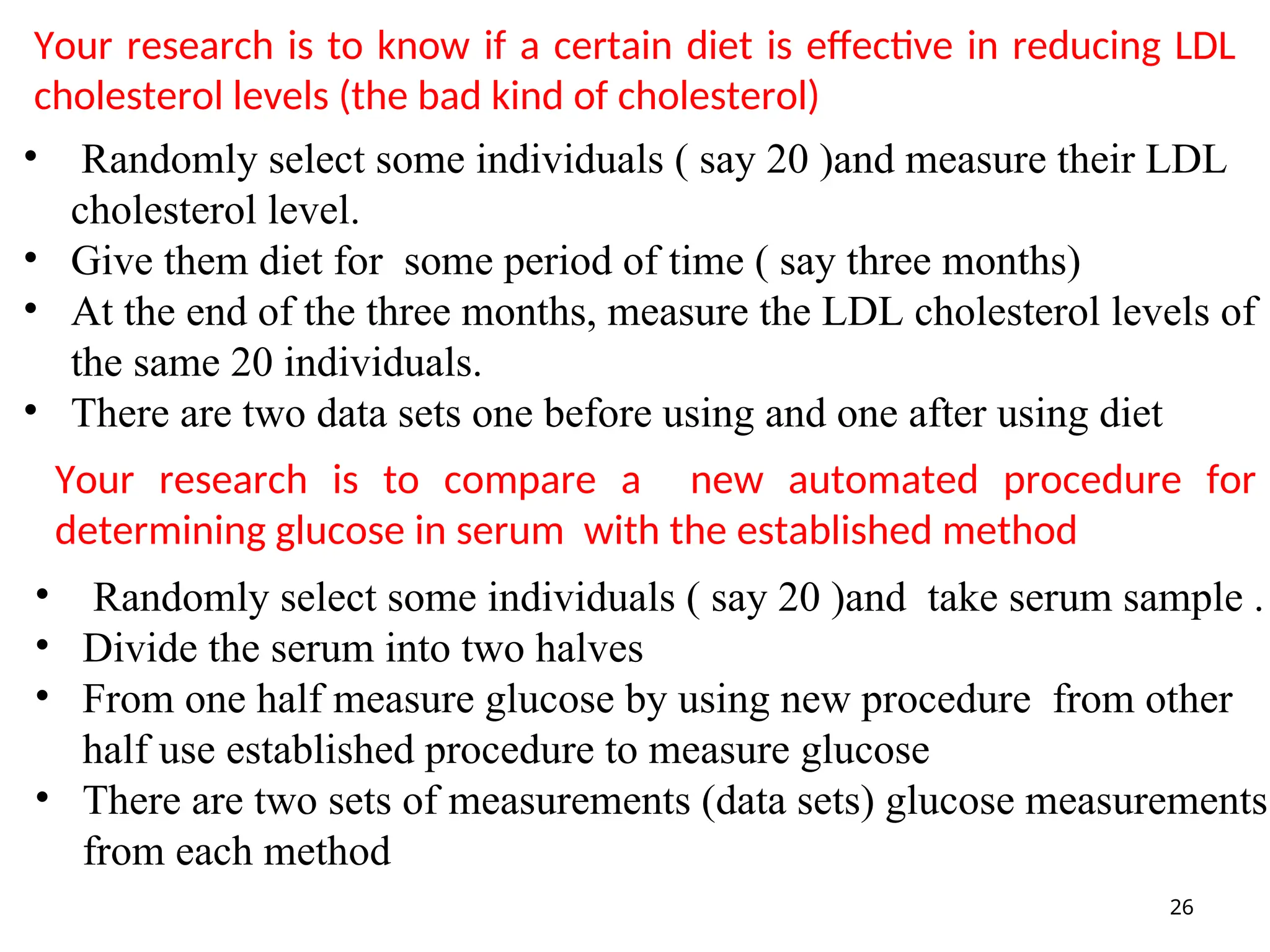
Your research is to know if a certain diet is effective in reducing LDL
cholesterol levels (the bad kind of cholesterol)
26
• Randomly select some individuals ( say 20 )and measure their LDL
cholesterol level.
• Give them diet for some period of time ( say three months)
• At the end of the three months, measure the LDL cholesterol levels of
the same 20 individuals.
• There are two data sets one before using and one after using diet
Your research is to compare a new automated procedure for
determining glucose in serum with the established method
• Randomly select some individuals ( say 20 )and take serum sample .
• Divide the serum into two halves
• From one half measure glucose by using new procedure from other
half use established procedure to measure glucose
• There are two sets of measurements (data sets) glucose measurements
from each method

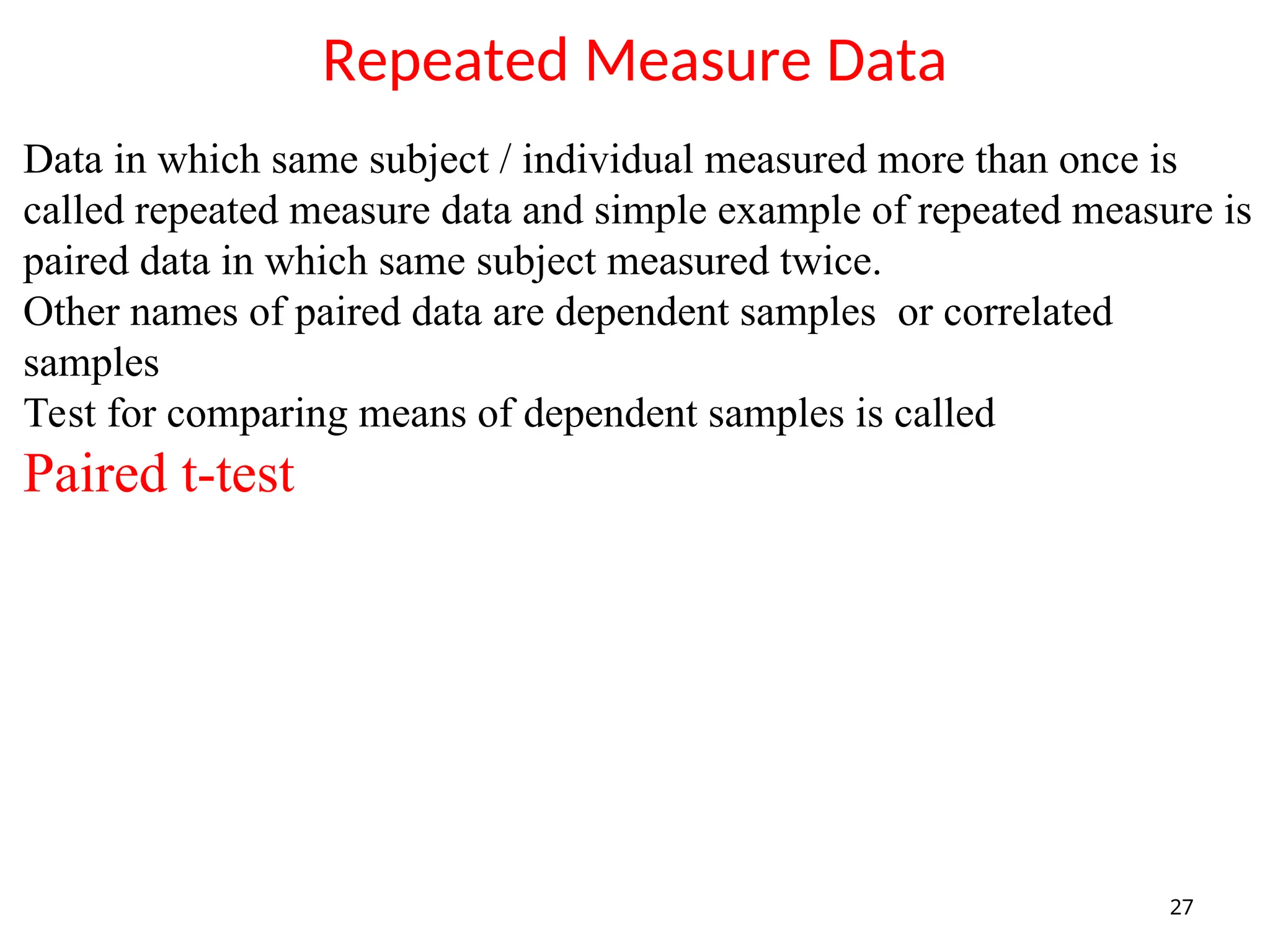
Repeated Measure Data
27
Data in which same subject / individual measured more than once is
called repeated measure data and simple example of repeated measure is
paired data in which same subject measured twice.
Other names of paired data are dependent samples or correlated
samples
Test for comparing means of dependent samples is called
Paired t-test

28
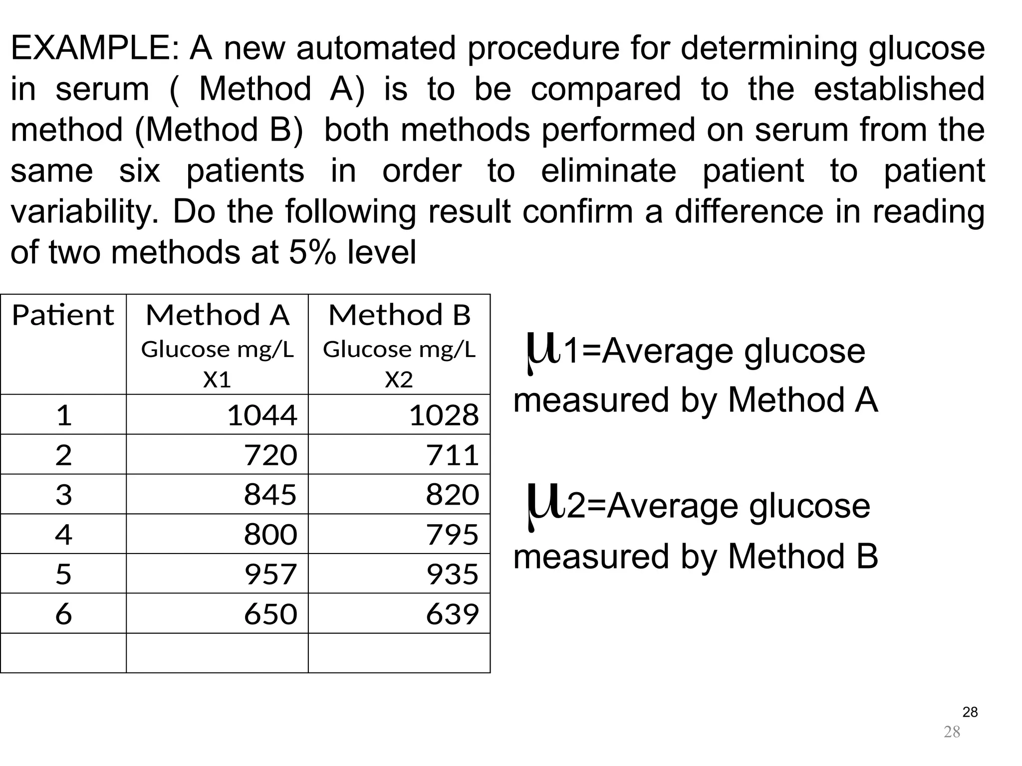
EXAMPLE: A new automated procedure for determining glucose
in serum ( Method A) is to be compared to the established
method (Method B) both methods performed on serum from the
same six patients in order to eliminate patient to patient
variability. Do the following result confirm a difference in reading
of two methods at 5% level
1=Average glucose
measured by Method A
2=Average glucose
measured by Method B
Patient Method A
Glucose mg/L
X1
Method B
Glucose mg/L
X2
1 1044 1028
2 720 711
3 845 820
4 800 795
5 957 935
6 650 639
28

29
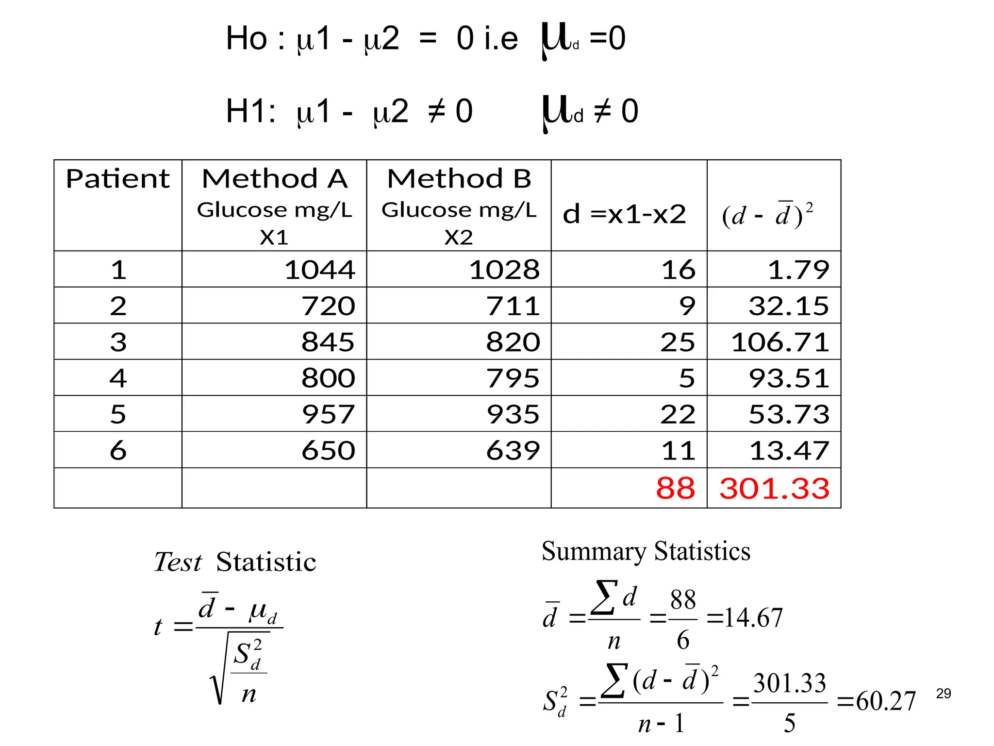
Ho : 1 - 2 = 0 i.e d =0
H1: 1 - 2 ≠ 0 d ≠ 0
Patient Method A
Glucose mg/L
X1
Method B
Glucose mg/L
X2
d =x1-x2 2
)
( d
d 
1 1044 1028 16 1.79
2 720 711 9 32.15
3 845 820 25 106.71
4 800 795 5 93.51
5 957 935 22 53.73
6 650 639 11 13.47
88 301.33
27
.
60
5
33
.
301
1
)
(
67
.
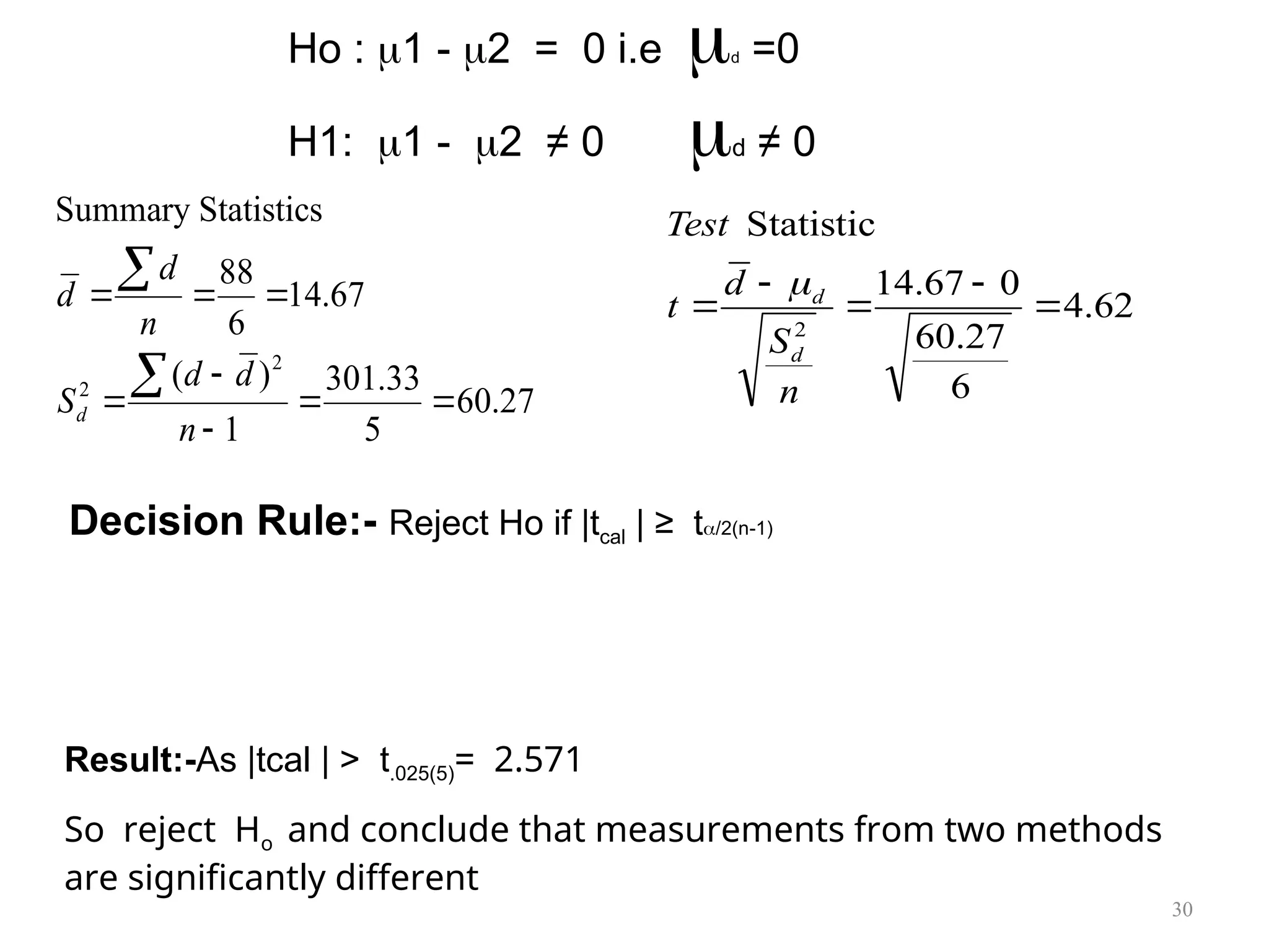
14
6
88
Statistics
Summary
2
2










n
d
d
S
n
d
d
d
n
S
d
t
Test
d
d
2
Statistic




Ho : 1 - 2 = 0 i.e d =0
H1: 1 - 2 ≠ 0 d ≠ 0
27
.
60
5
33
.
301
1
)
(
67
.
14
6
88
Statistics
Summary
2
2










n
d
d
S
n
d
d
d
62
.
4
6
27
.
60
0
67
.
14
Statistic
2





n
S
d
t
Test
d
d

Decision Rule:- Reject Ho if |tcal | ≥ t/2(n-1)
Result:-As |tcal | > t.025(5)= 2.571
So reject Ho and conclude that measurements from two methods
are significantly different
30

Percentage points of t distribution
df 0.1 0.05 0.025 0.005 0.001 0.0005
1 3.078 6.314 12.706 63.657 318.309 636.619
2 1.886 2.920 4.303 9.925 22.327 31.599
3 1.638 2.353 3.182 5.841 10.215 12.924
4 1.533 2.132 2.776 4.604 7.173 8.610
5 1.476 2.015 2.571 4.032 5.893 6.869
6 1.440 1.943 2.447 3.707 5.208 5.959
7 1.415 1.895 2.365 3.499 4.785 5.408
8 1.397 1.860 2.306 3.355 4.501 5.041
9 1.383 1.833 2.262 3.250 4.297 4.781
10 1.372 1.812 2.228 3.169 4.144 4.587
11 1.363 1.796 2.201 3.106 4.025 4.437
12 1.356 1.782 2.179 3.055 3.930 4.318
13 1.350 1.771 2.160 3.012 3.852 4.221
14 1.345 1.761 2.145 2.977 3.787 4.140
15 1.341 1.753 2.131 2.947 3.733 4.073
16 1.337 1.746 2.120 2.921 3.686 4.015
17 1.333 1.740 2.110 2.898 3.646 3.965
18 1.330 1.734 2.101 2.878 3.610 3.922
19 1.328 1.729 2.093 2.861 3.579 3.883
20 1.325 1.725 2.086 2.845 3.552 3.850
21 1.323 1.721 2.080 2.831 3.527 3.819
22 1.321 1.717 2.074 2.819 3.505 3.792
23 1.319 1.714 2.069 2.807 3.485 3.768
24 1.318 1.711 2.064 2.797 3.467 3.745
25 1.316 1.708 2.060 2.787 3.450 3.725
26 1.315 1.706 2.056 2.779 3.435 3.707
27 1.314 1.703 2.052 2.771 3.421 3.690
28 1.313 1.701 2.048 2.763 3.408 3.674
29 1.311 1.699 2.045 2.756 3.396 3.659
30 1.310 1.697 2.042 2.750 3.385 3.646
40 1.303 1.684 2.021 2.704 3.307 3.551
Table
31

5--Test of hypothesis statistics (part_1).ppt

More Related Content

Similar to 5--Test of hypothesis statistics (part_1).ppt

Recently uploaded

5--Test of hypothesis statistics (part_1).ppt