Downloaded 120 times
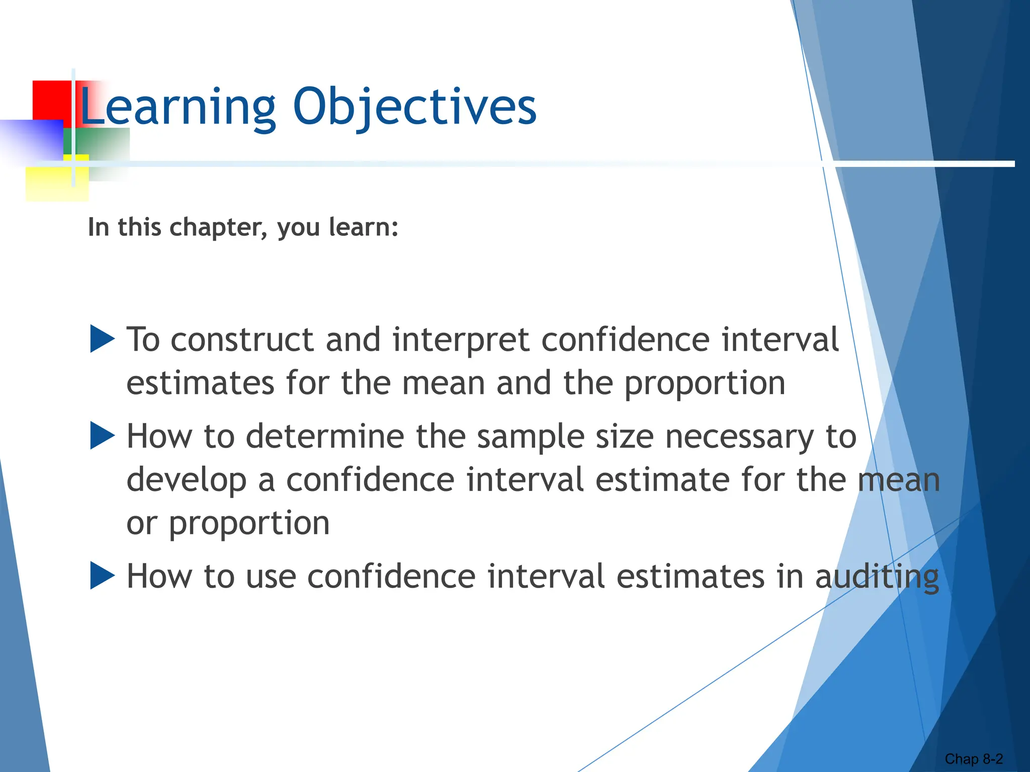
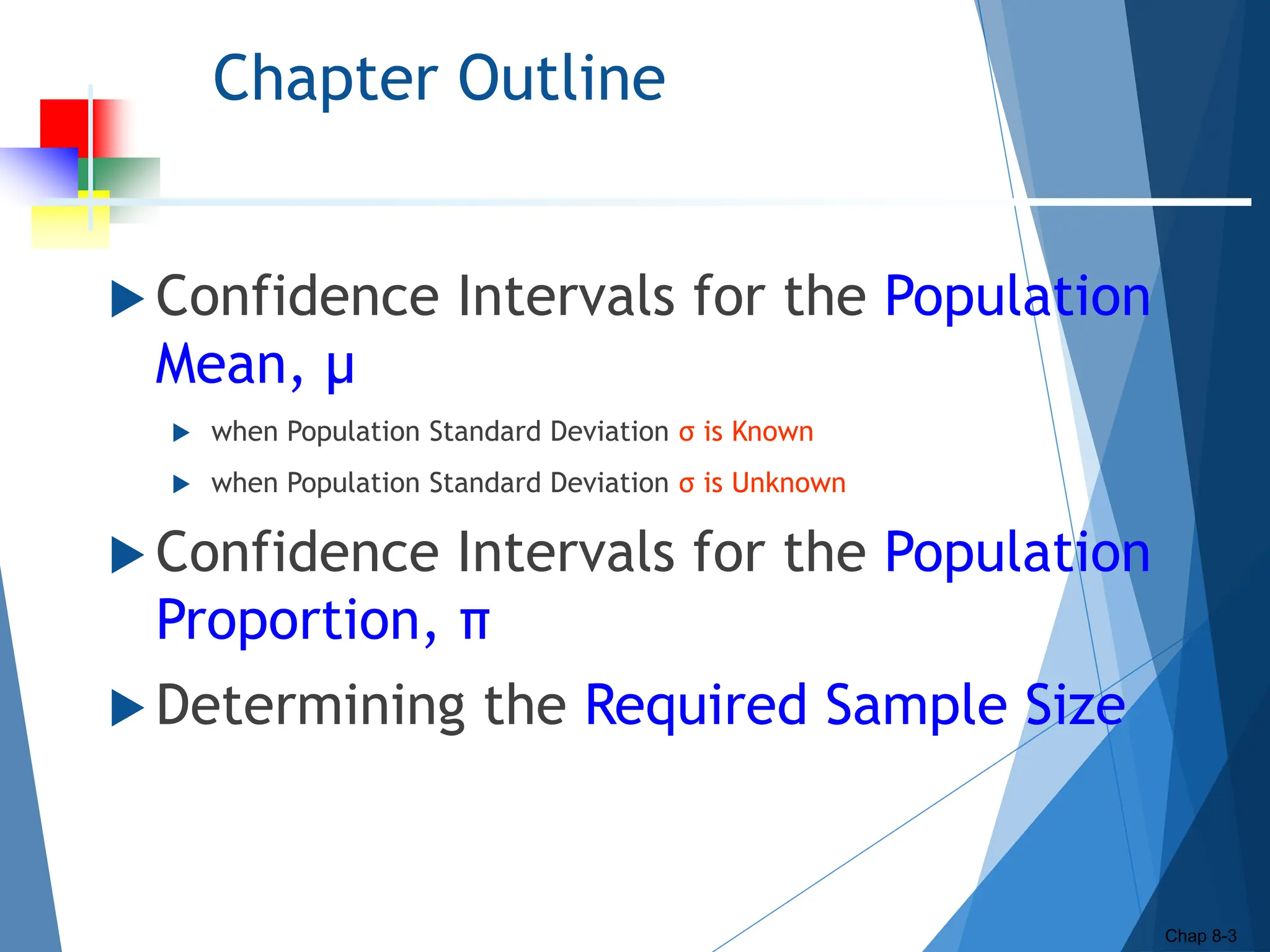
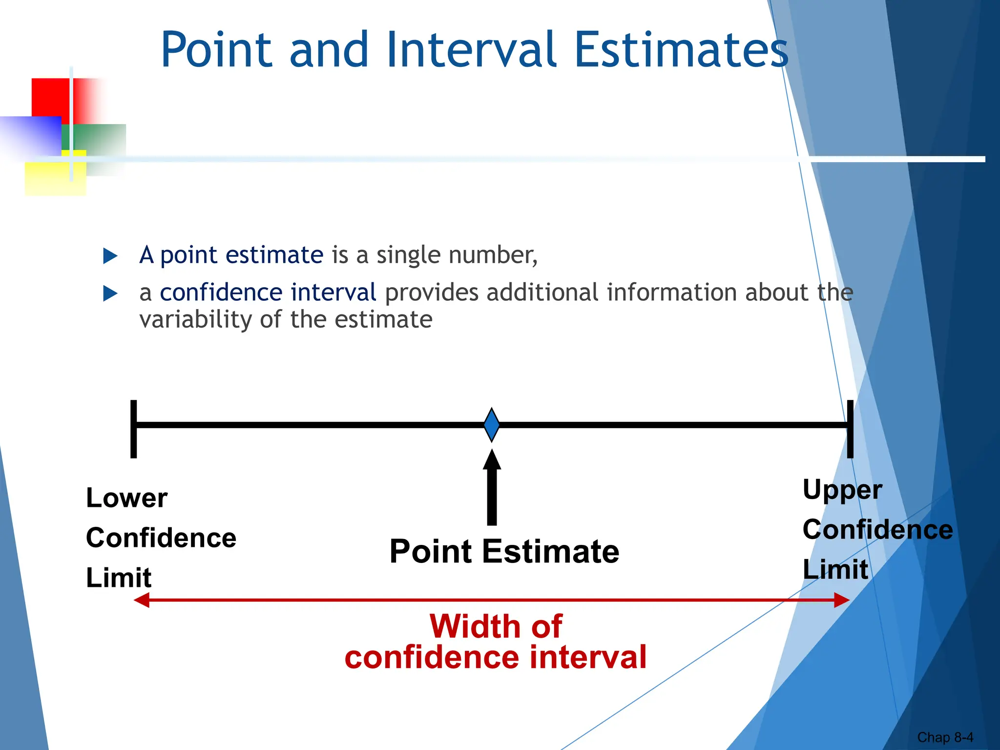
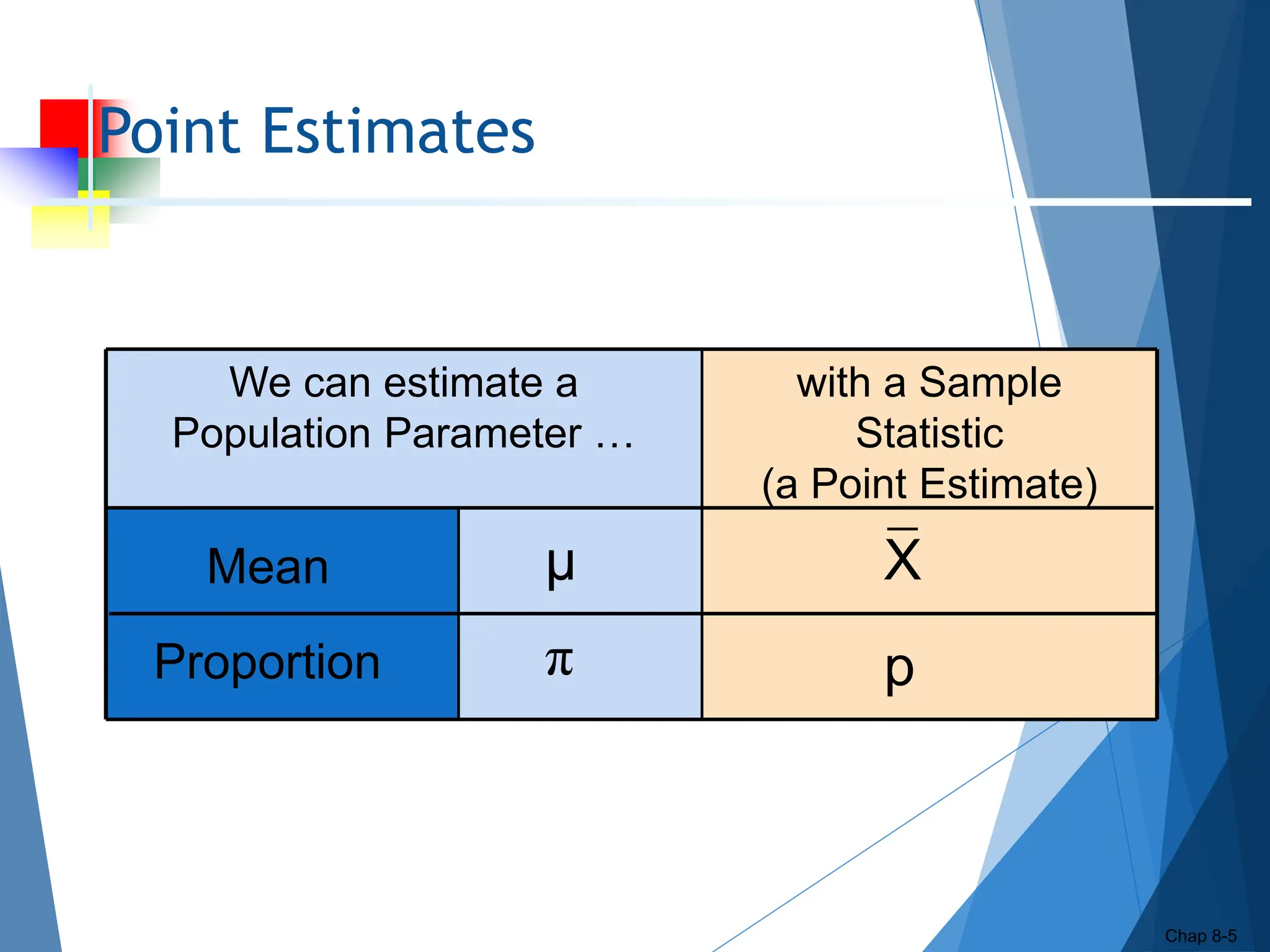
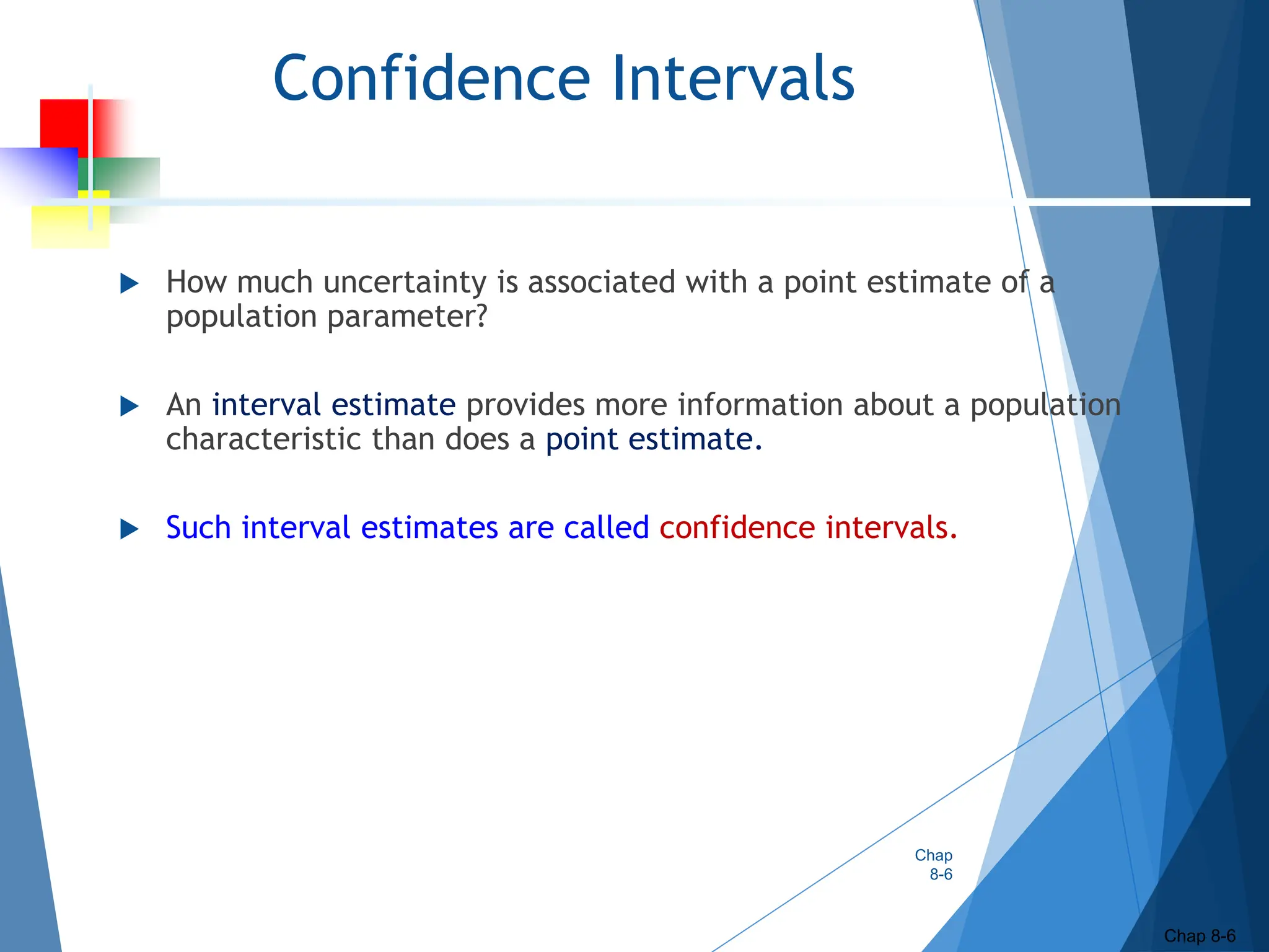
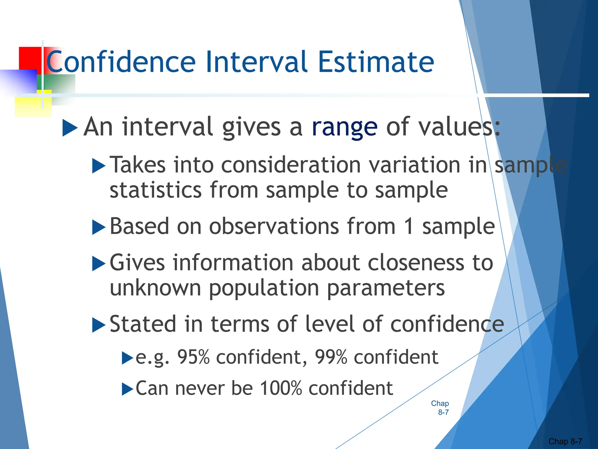
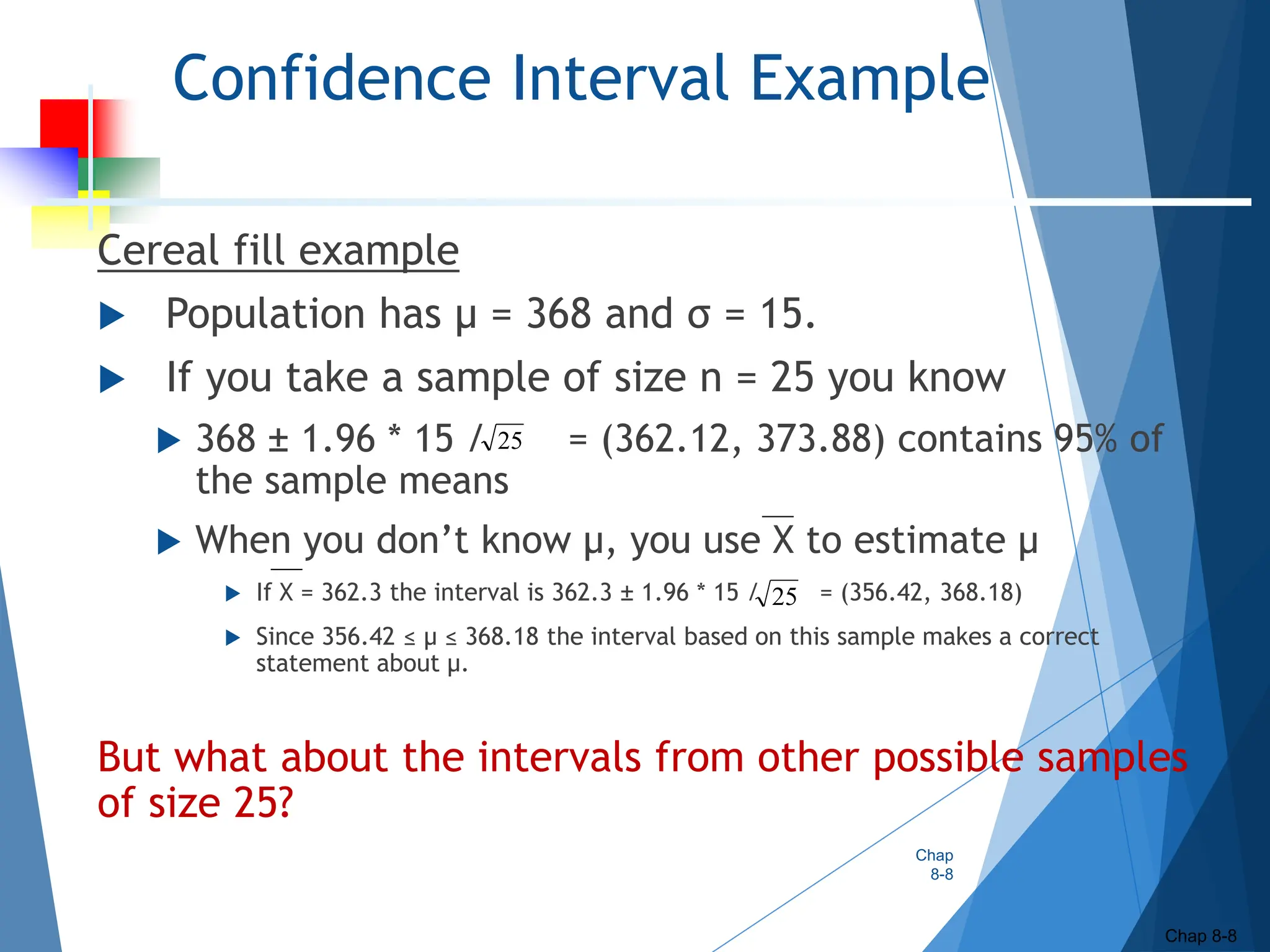
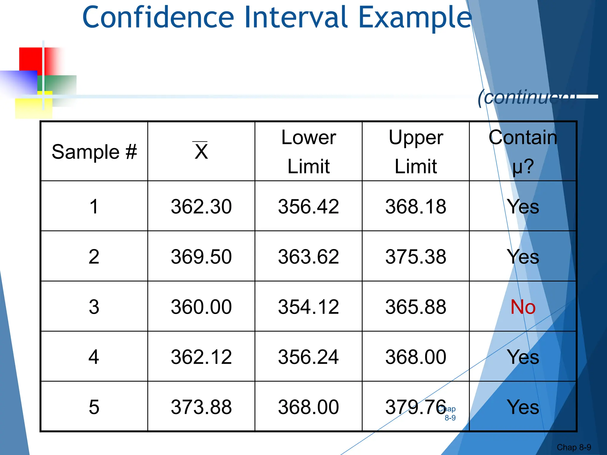
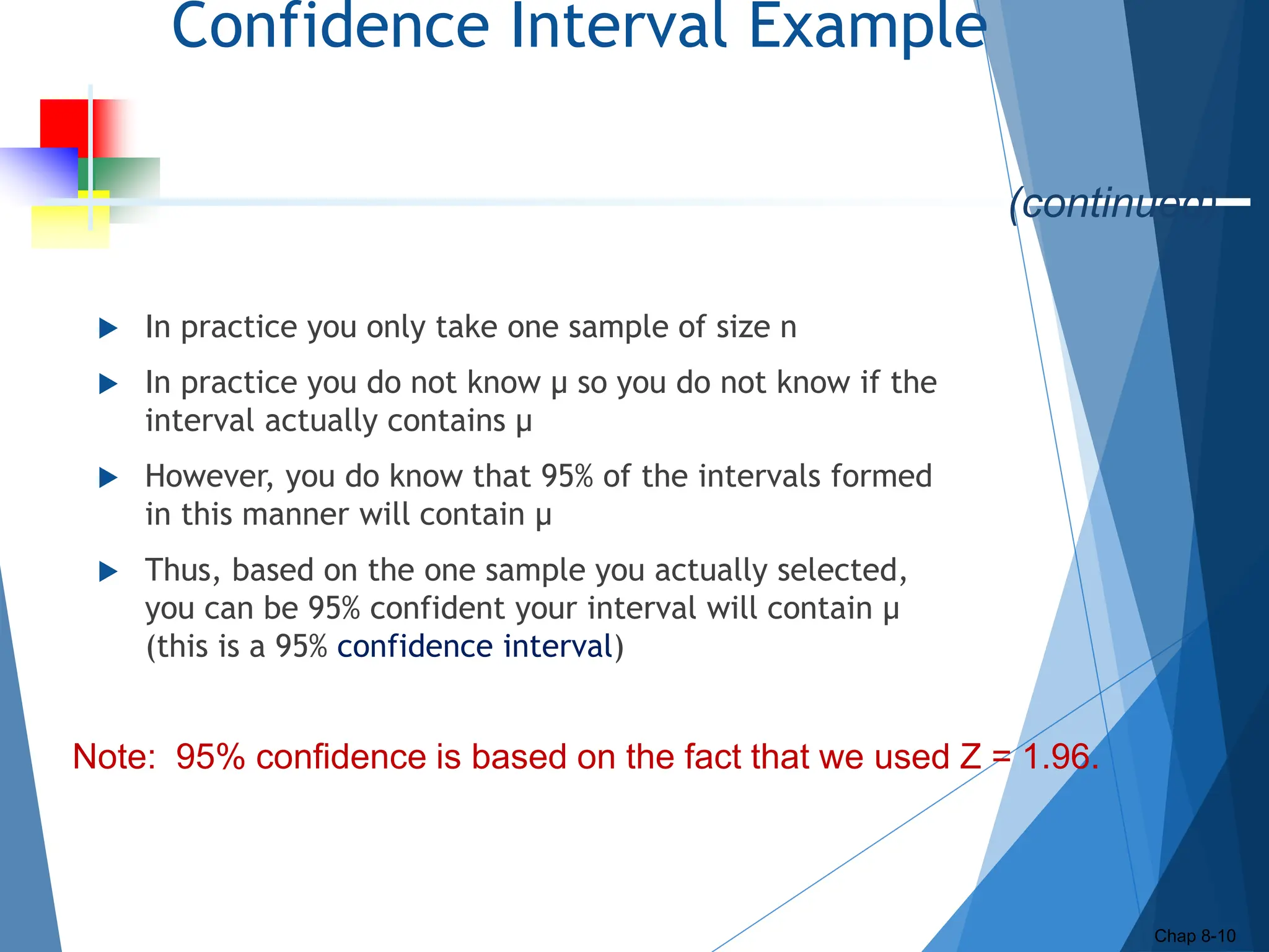
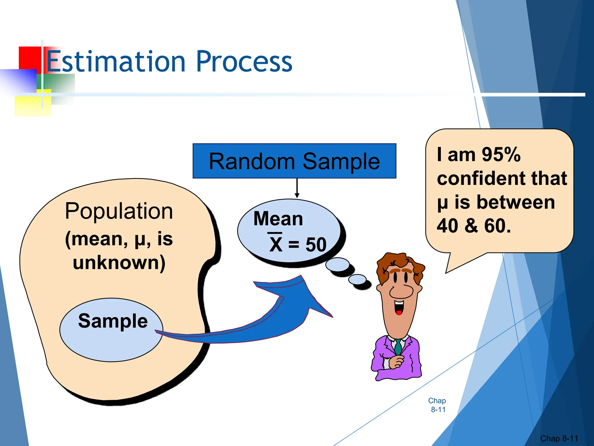
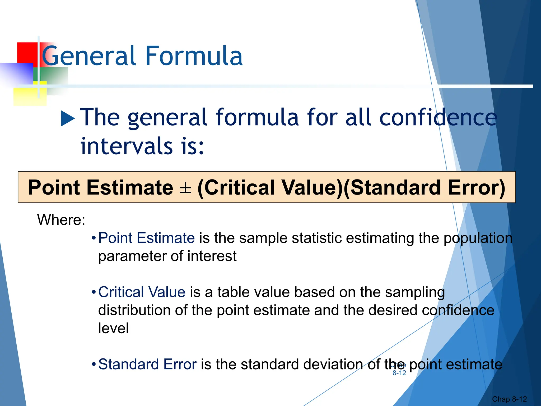
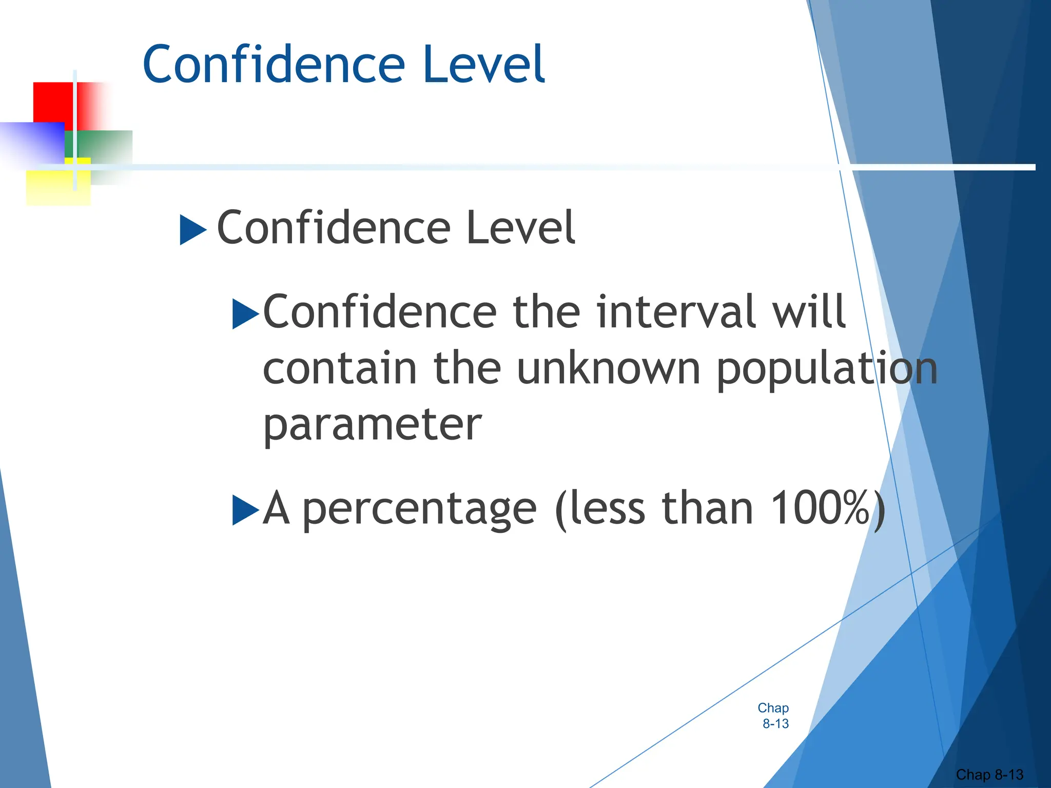
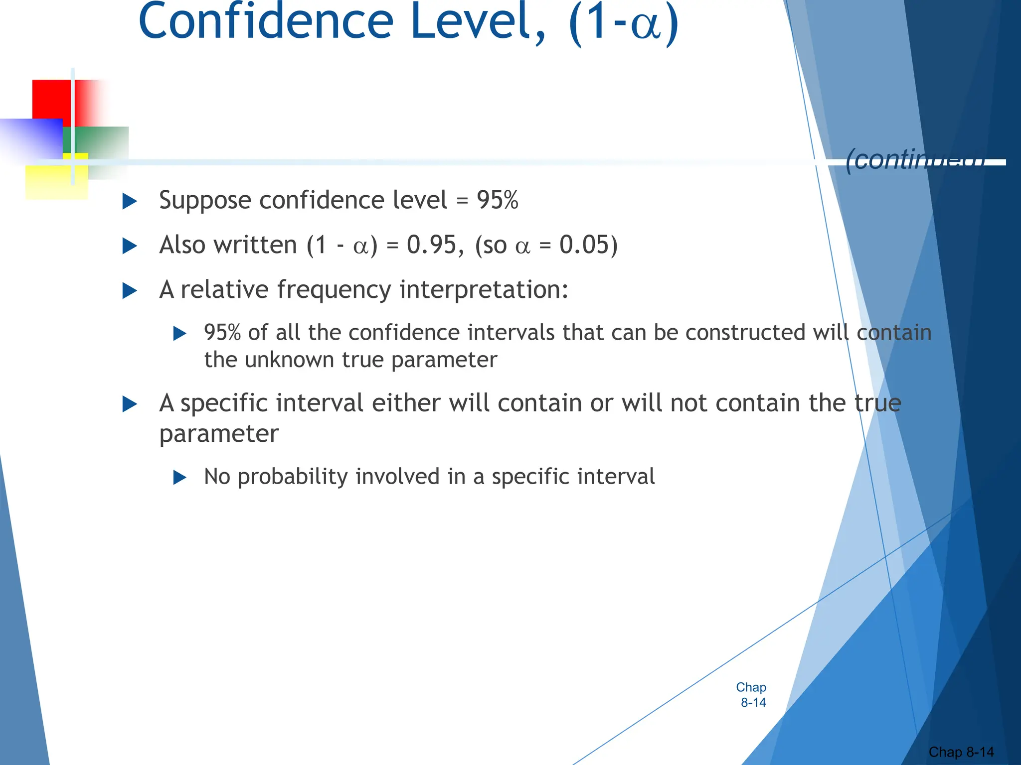
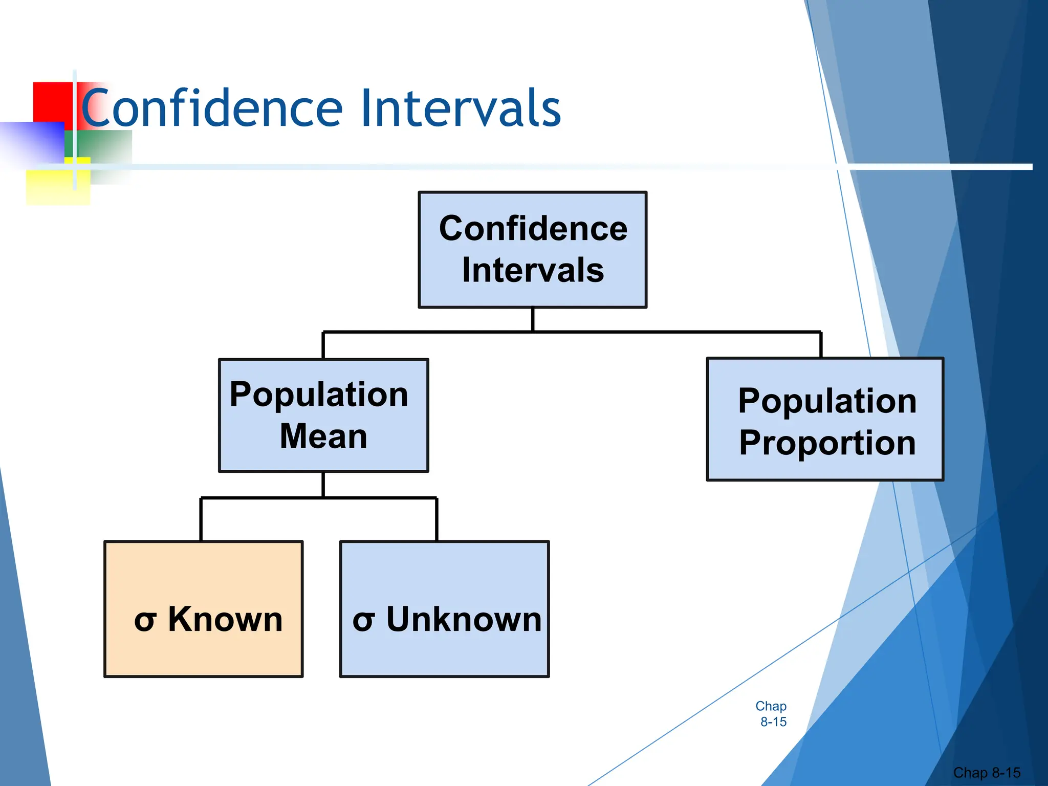
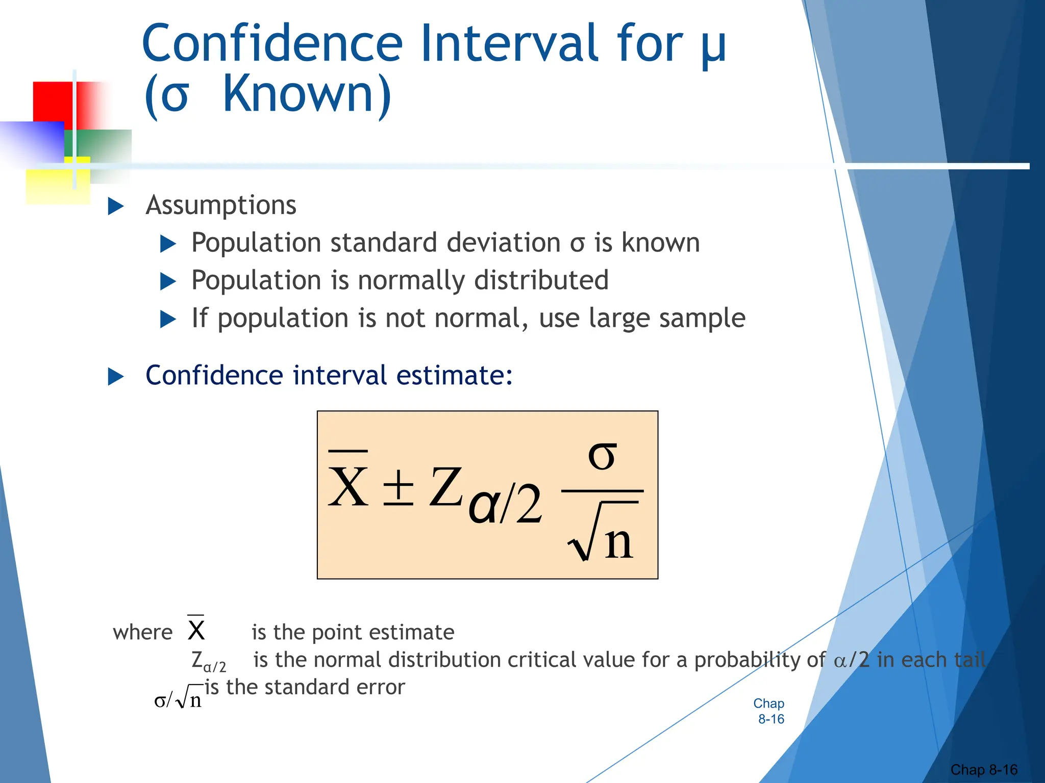
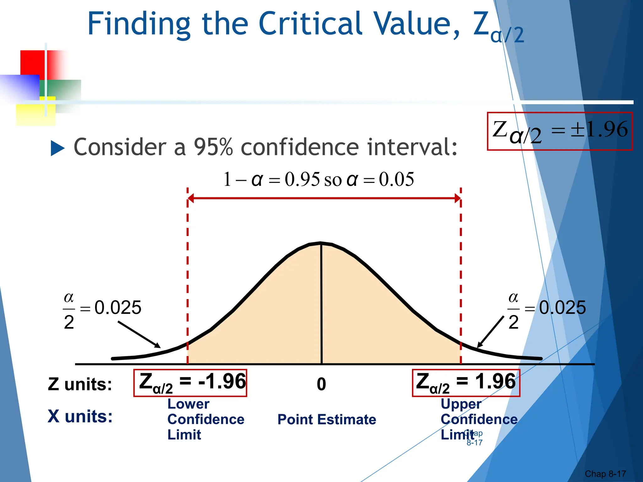
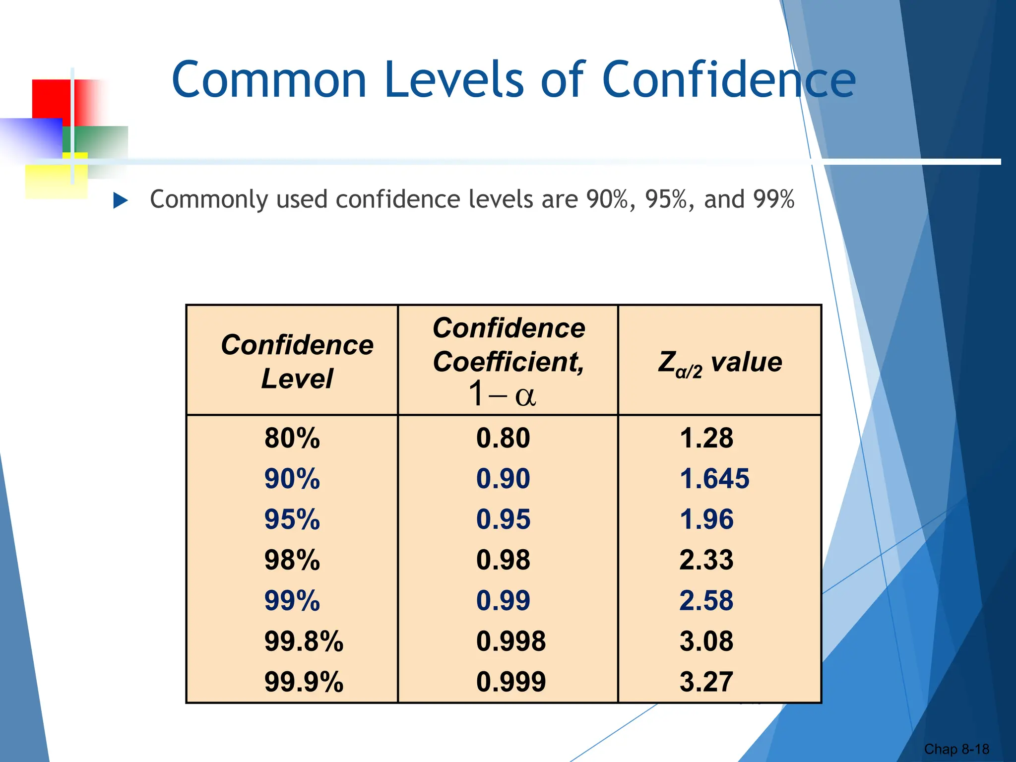
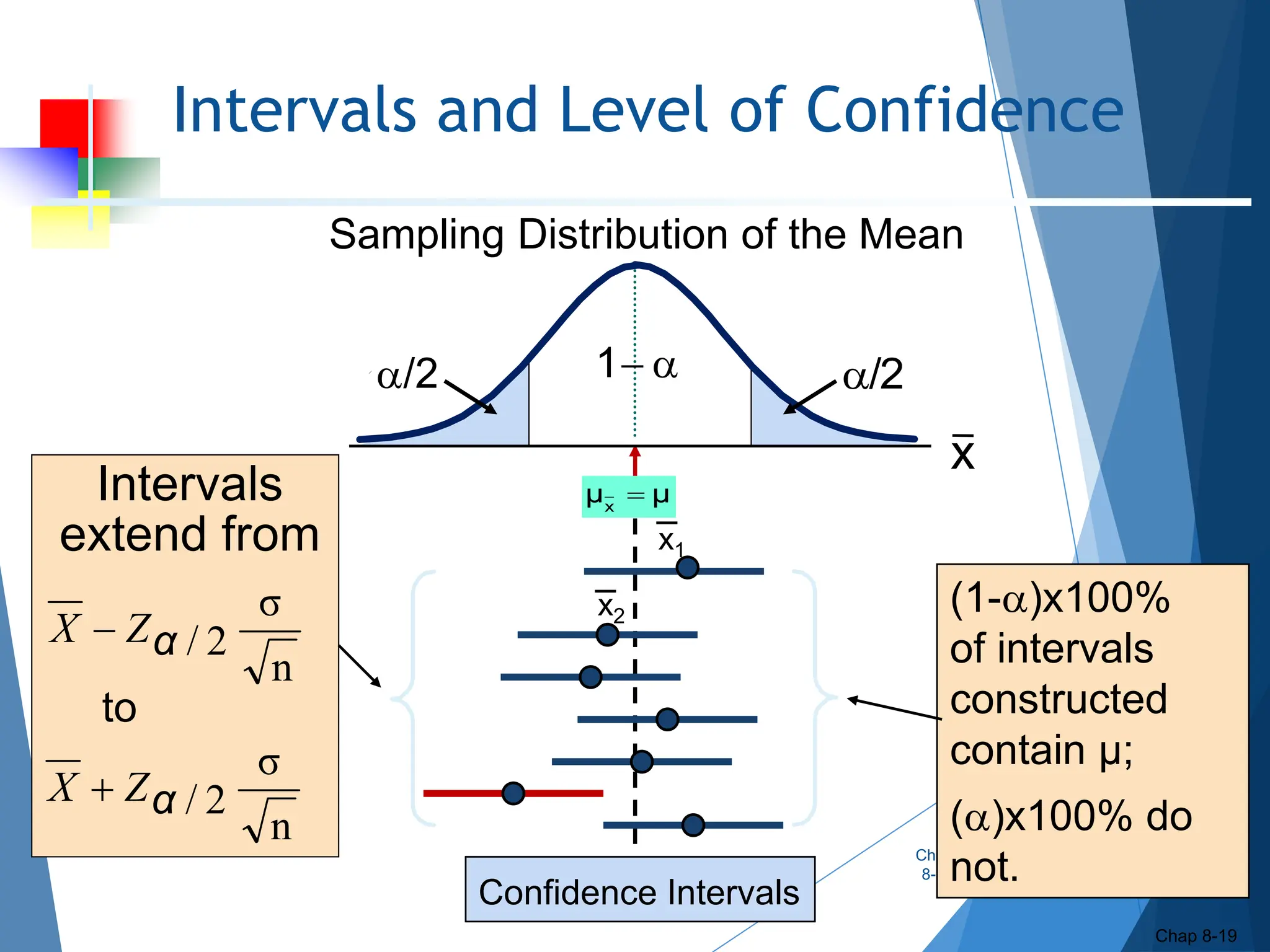
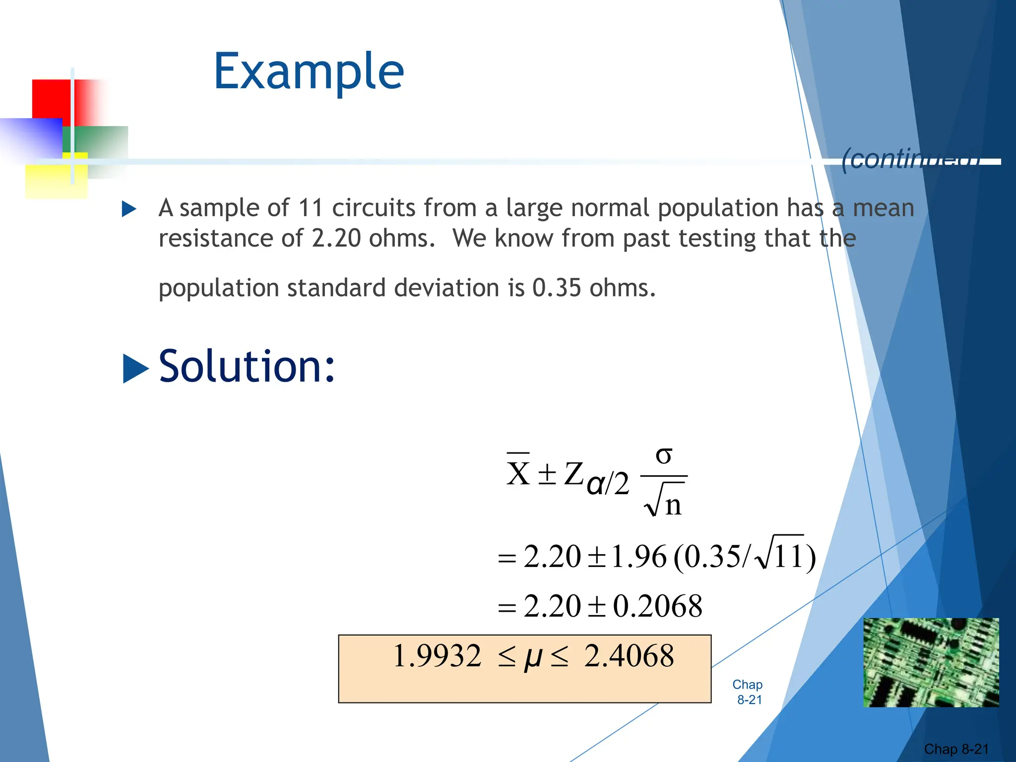
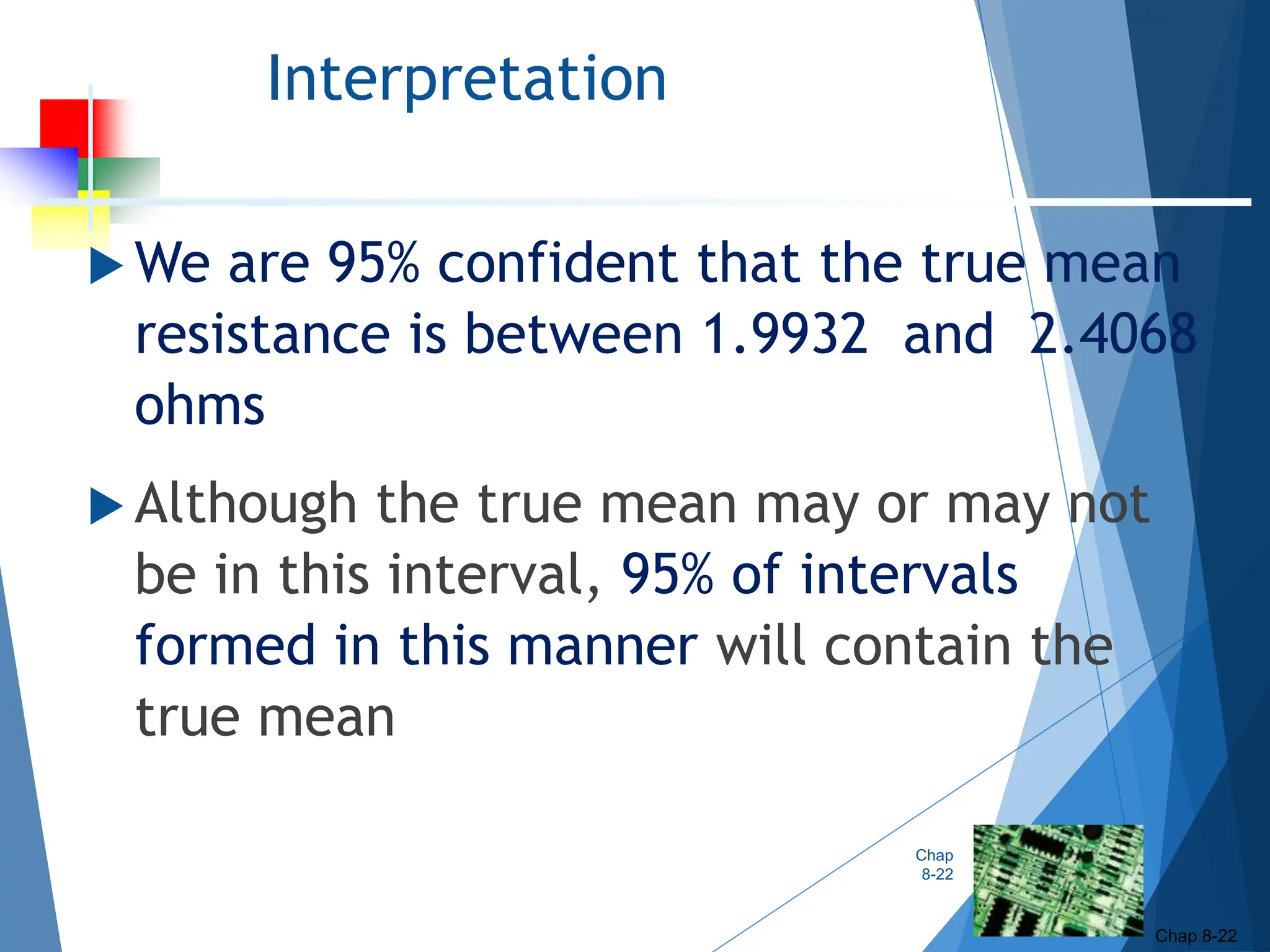
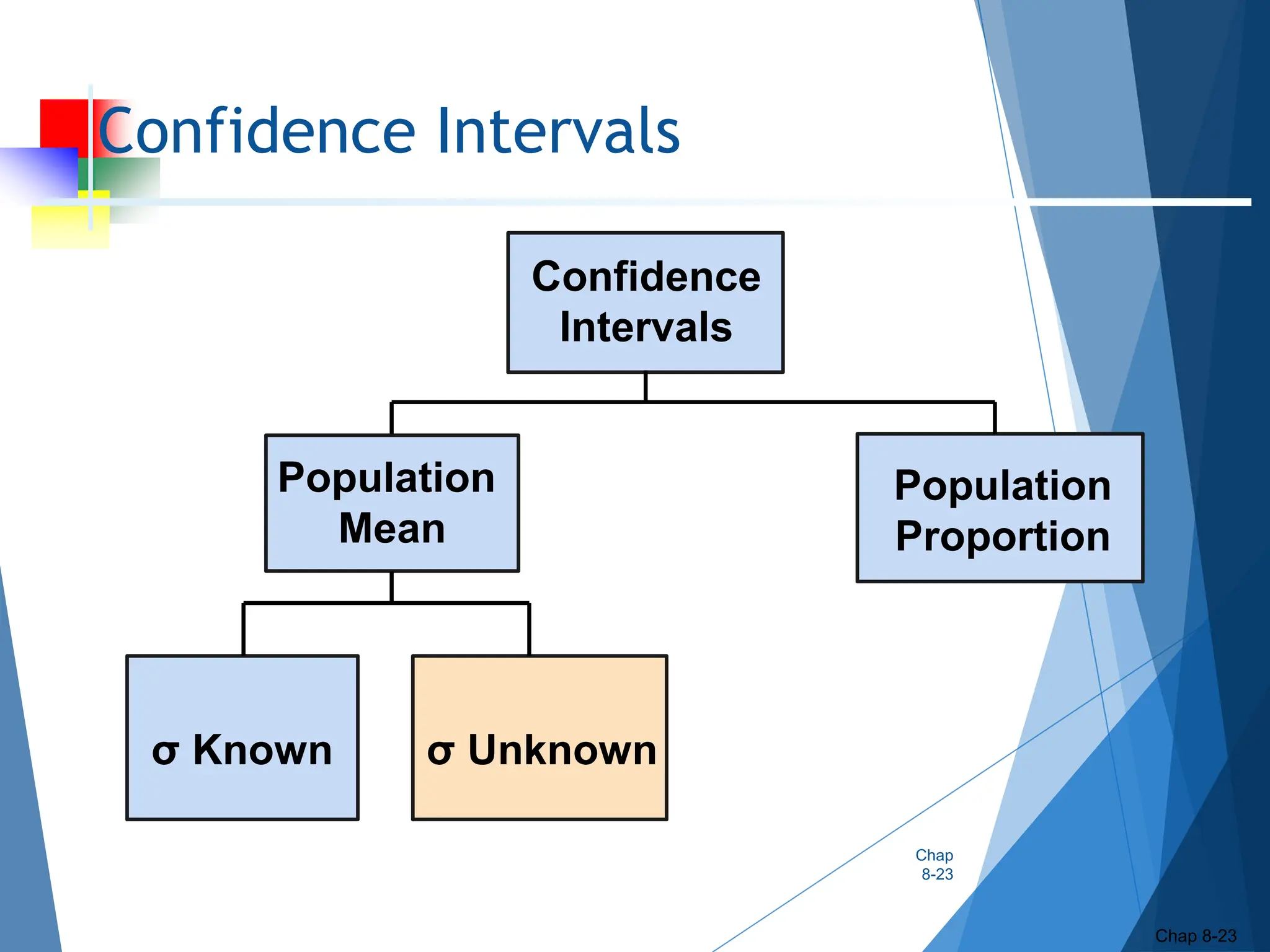
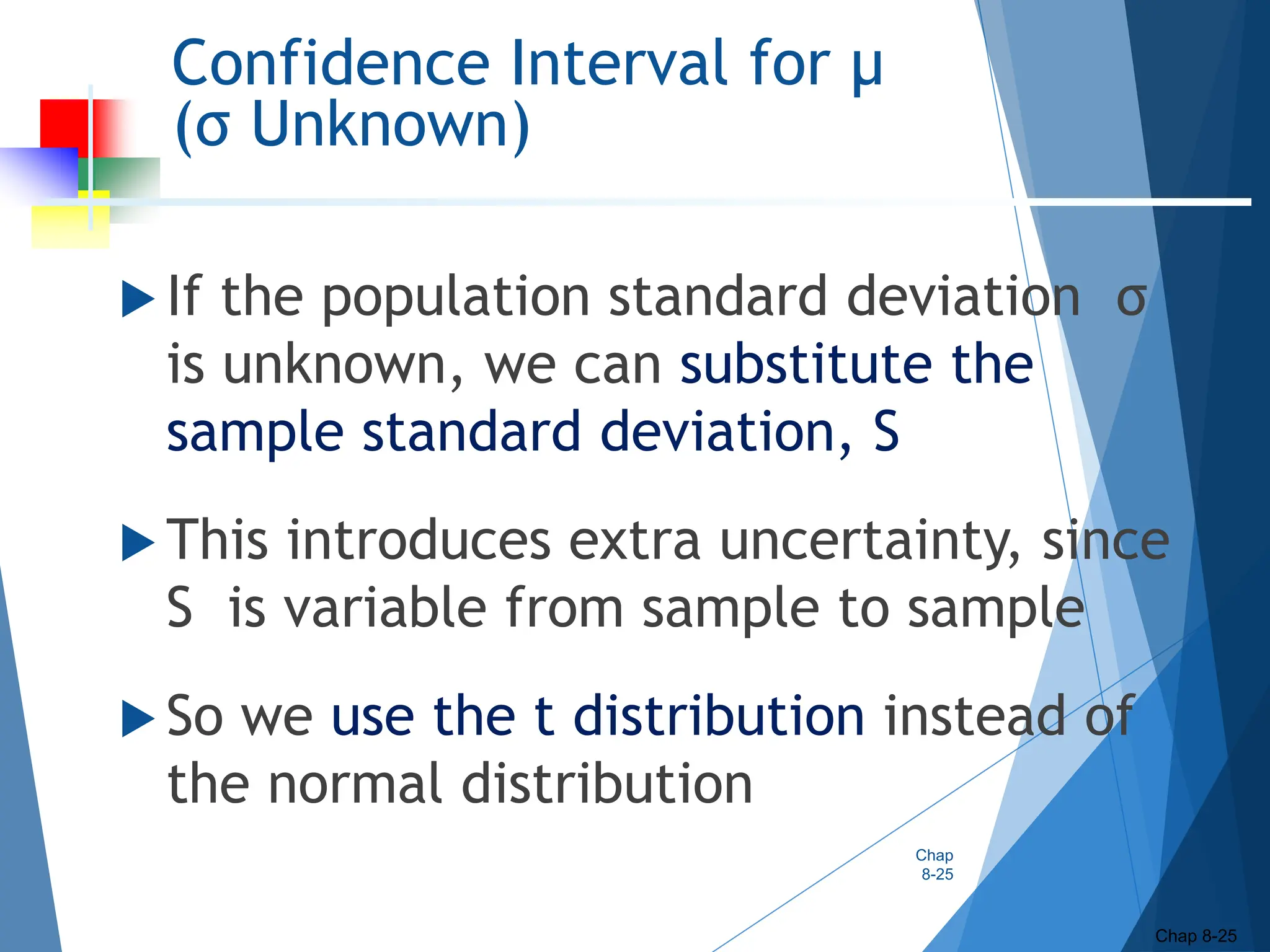
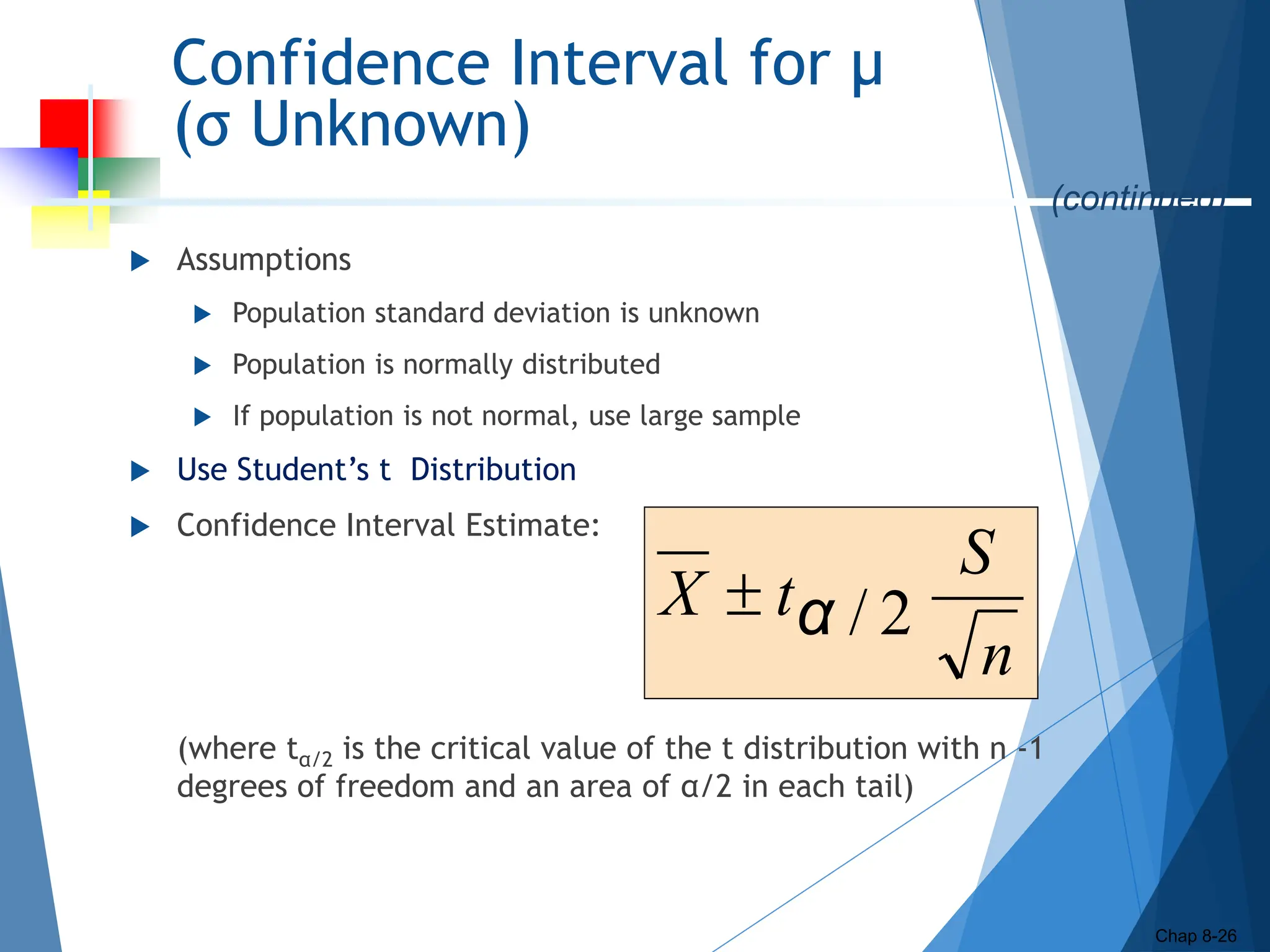
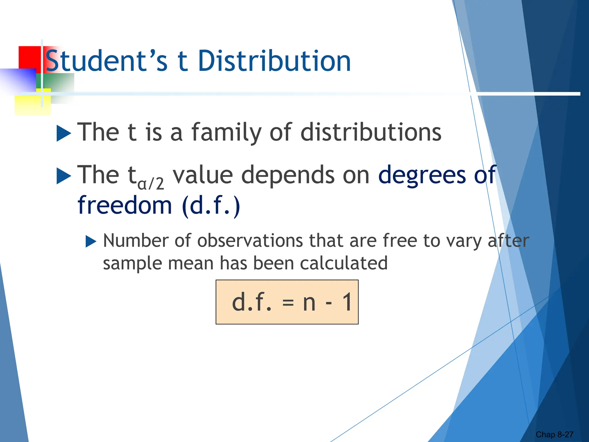
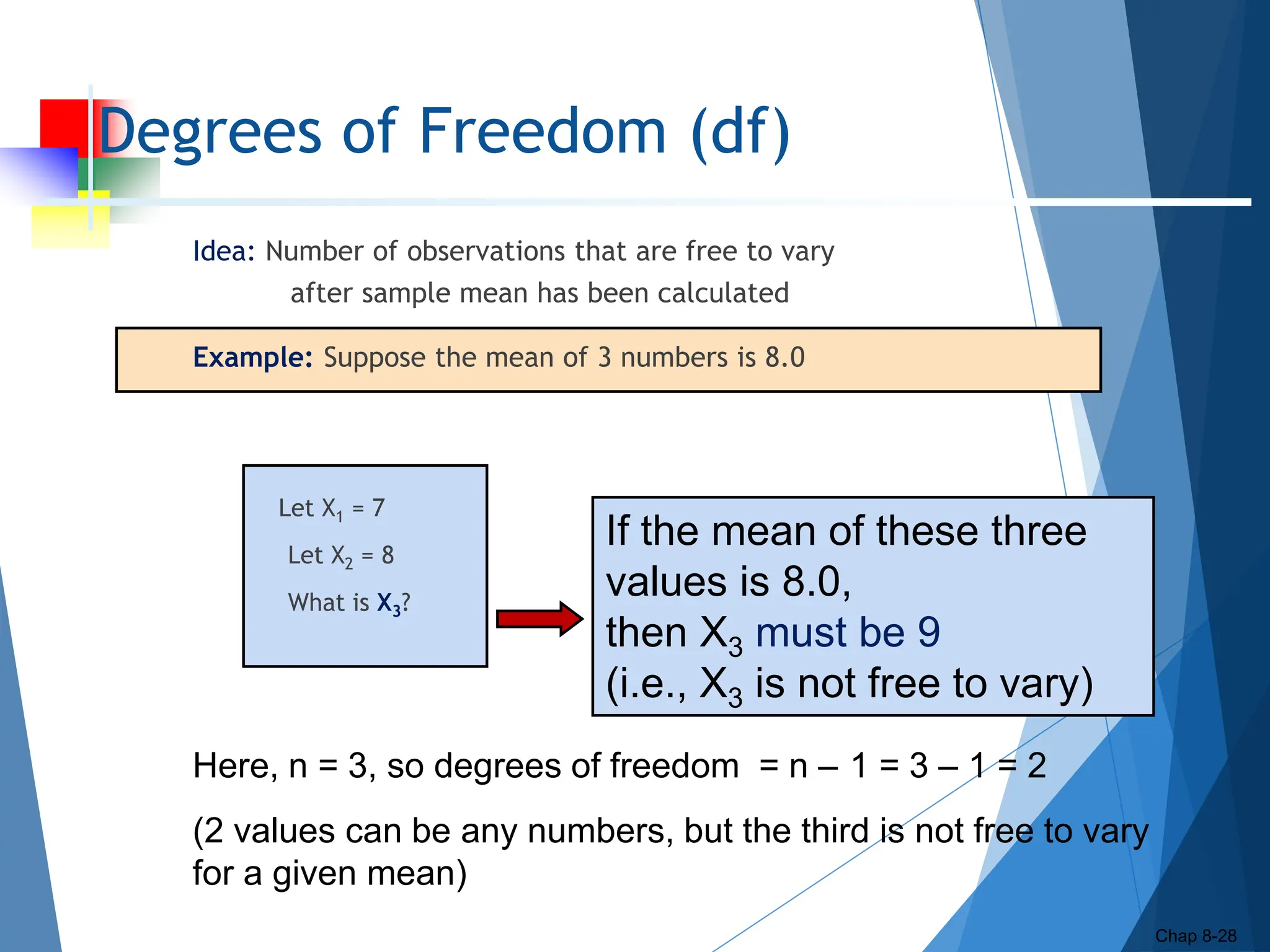
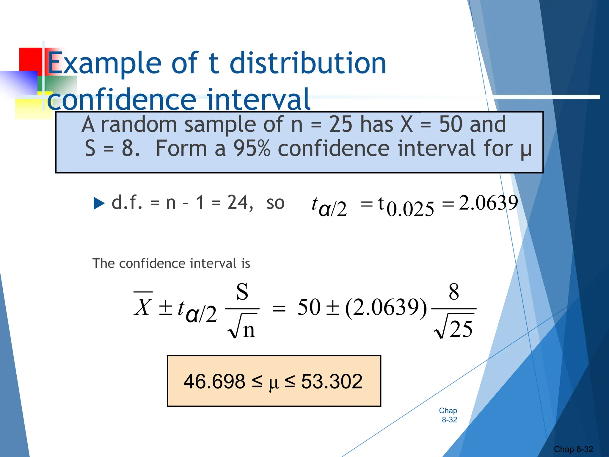

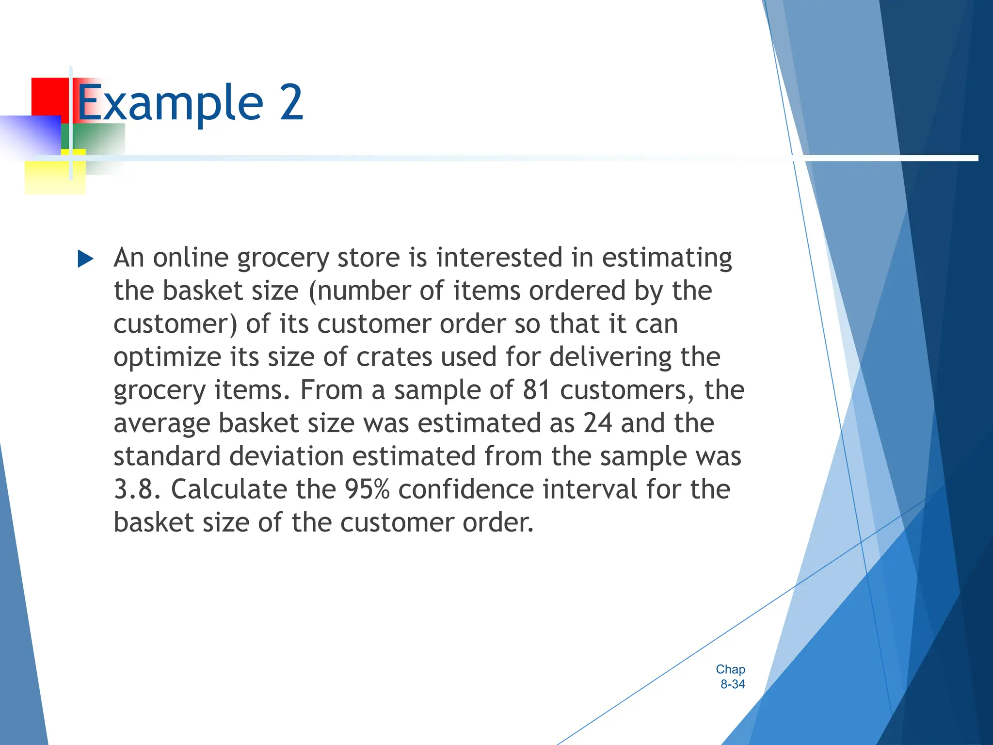
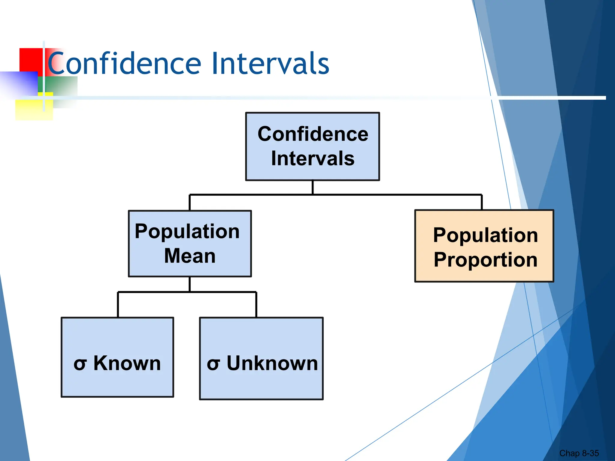
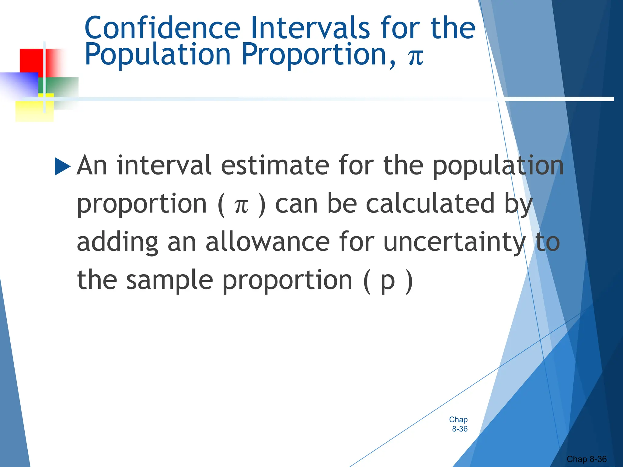
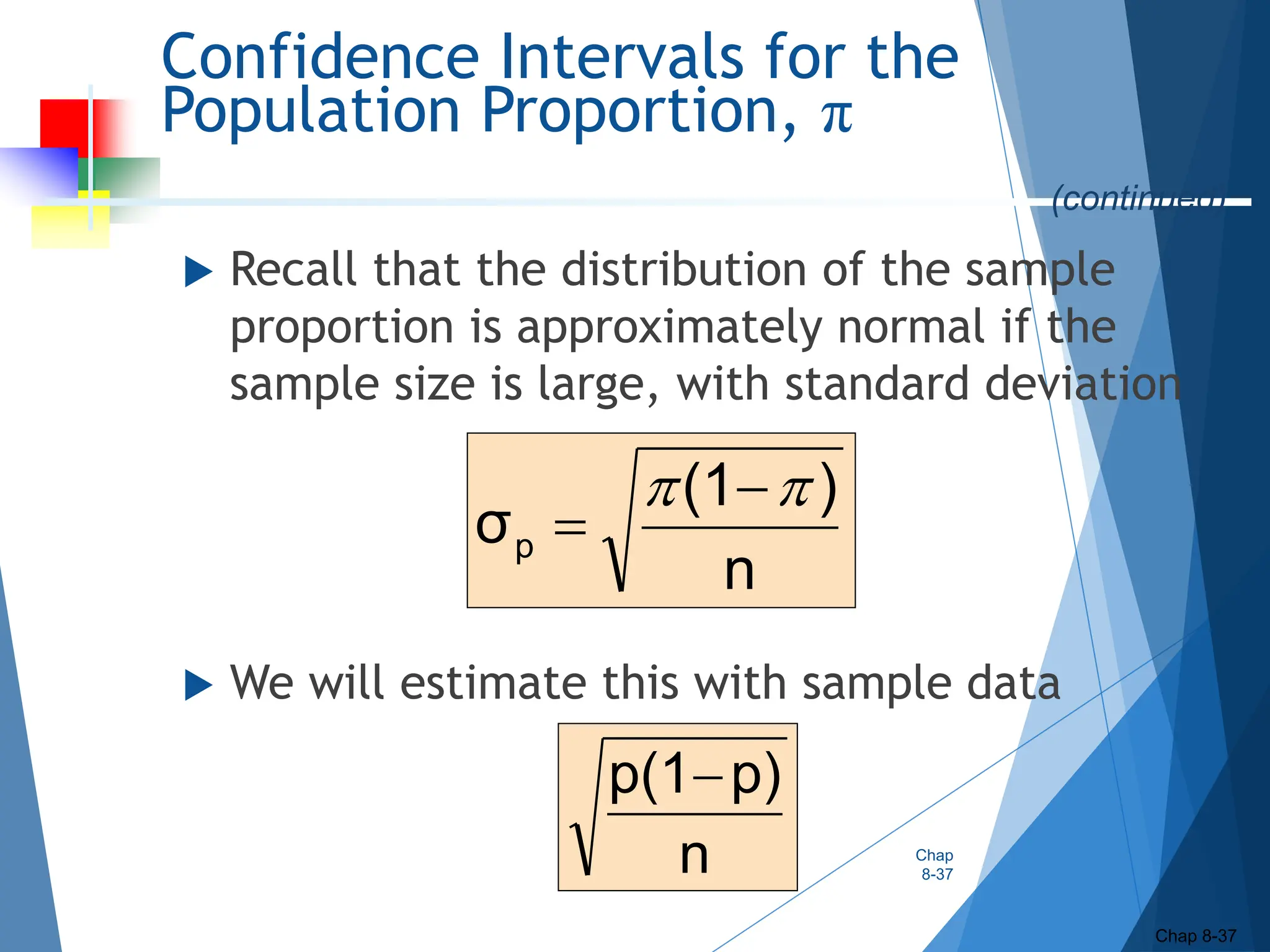
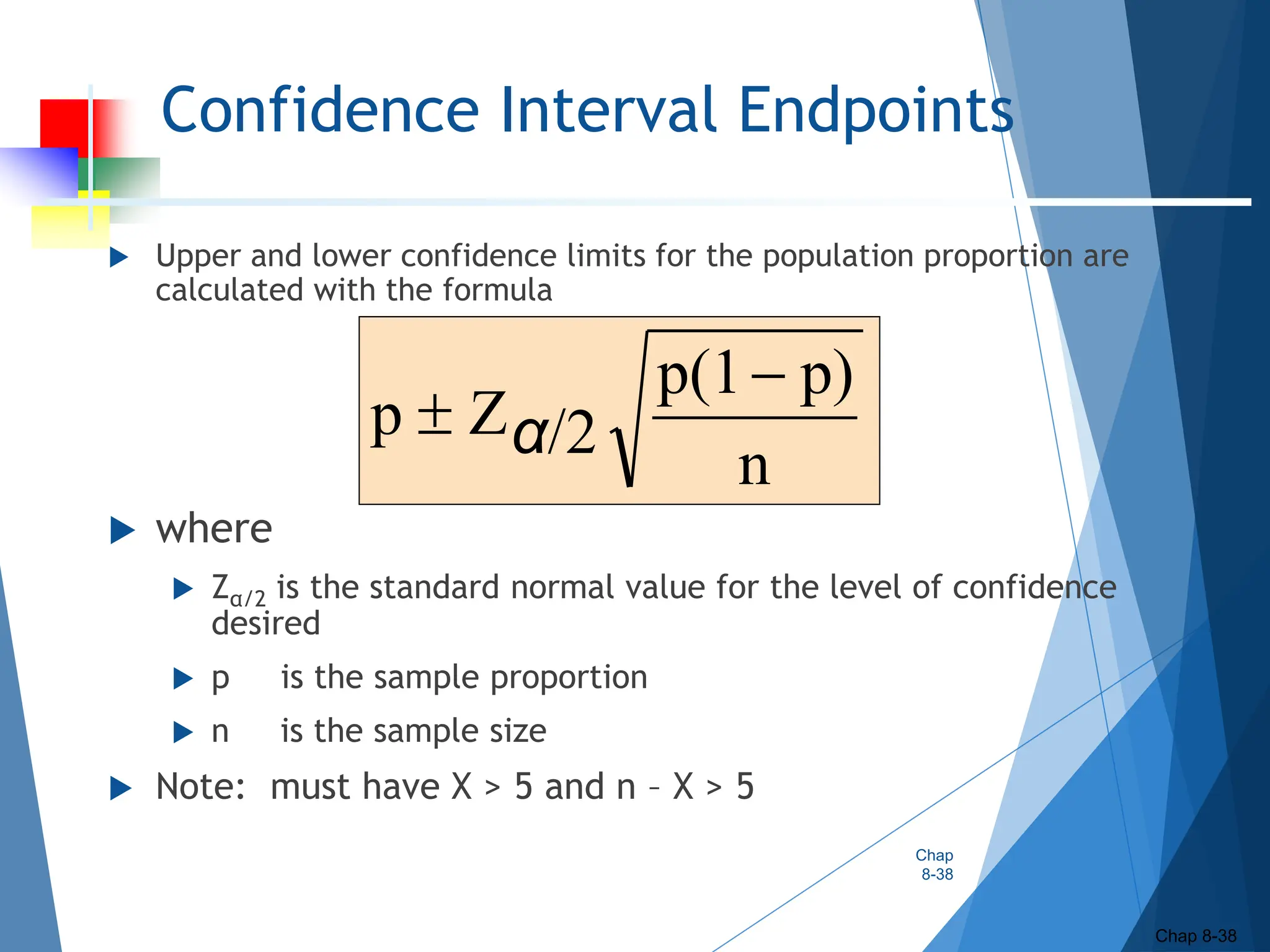
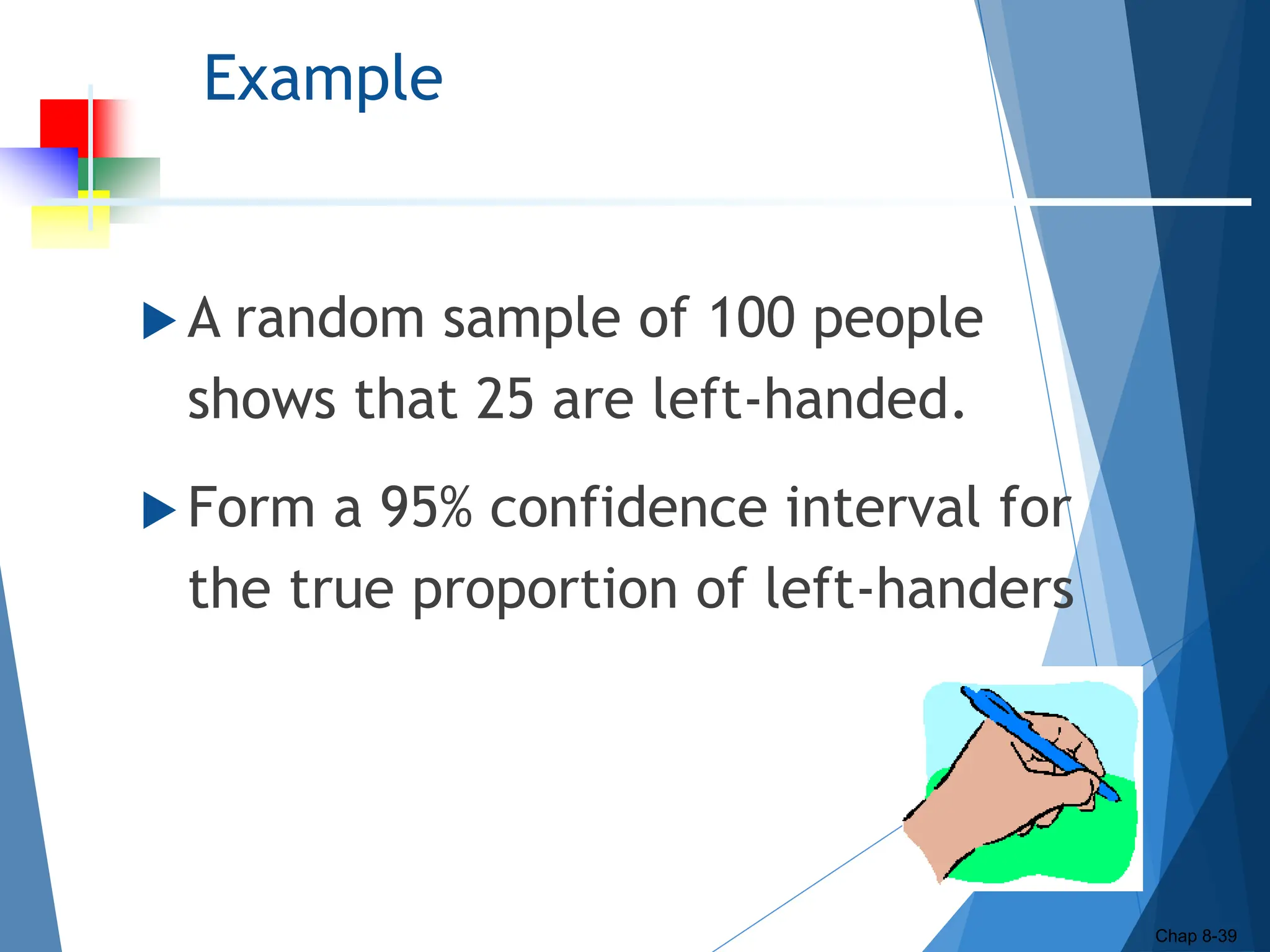
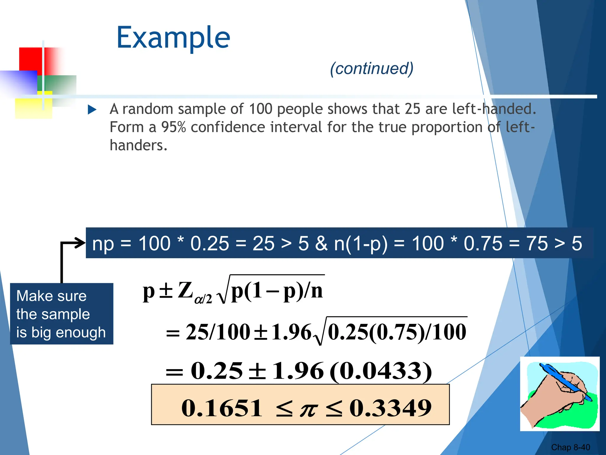
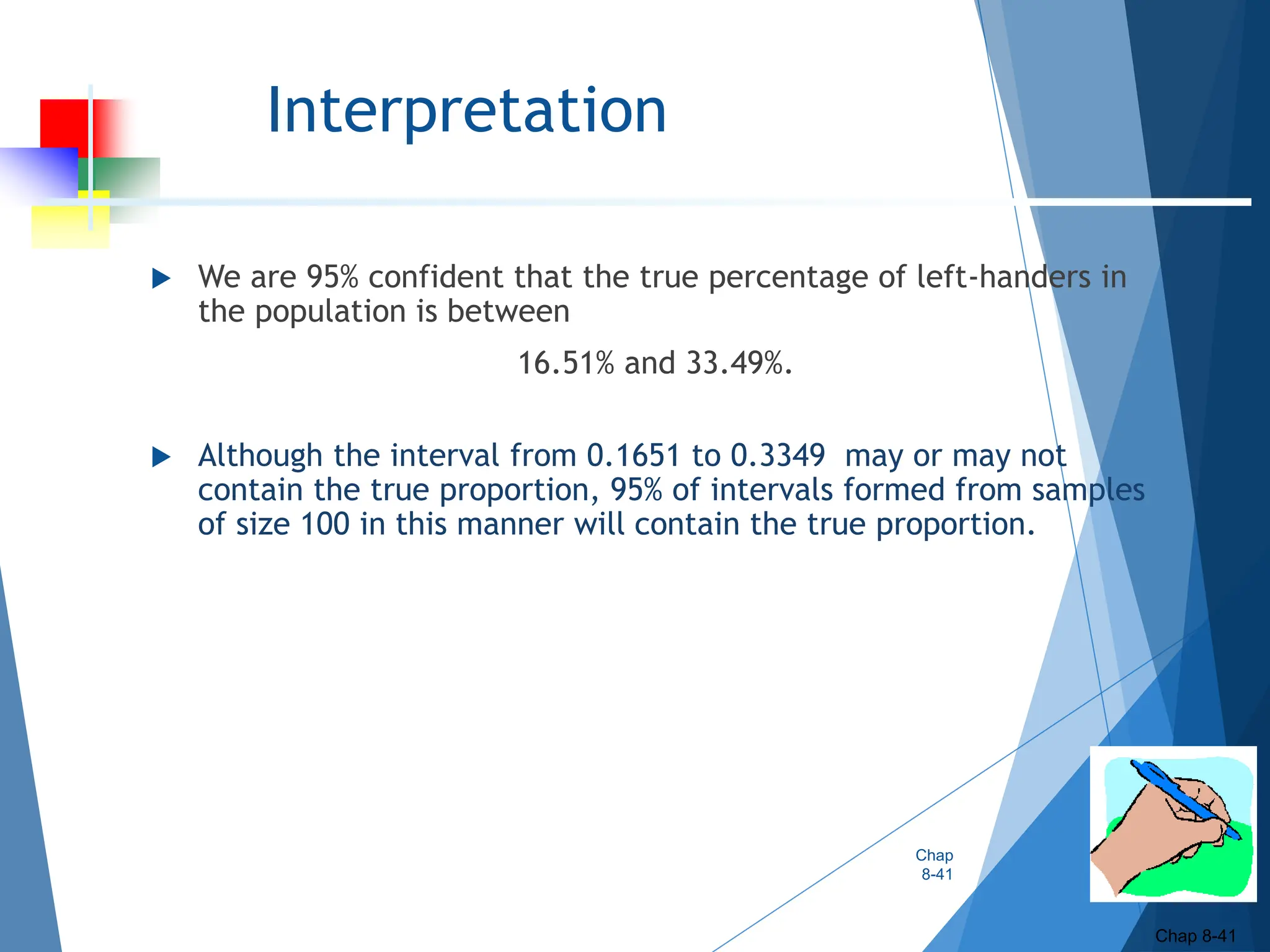

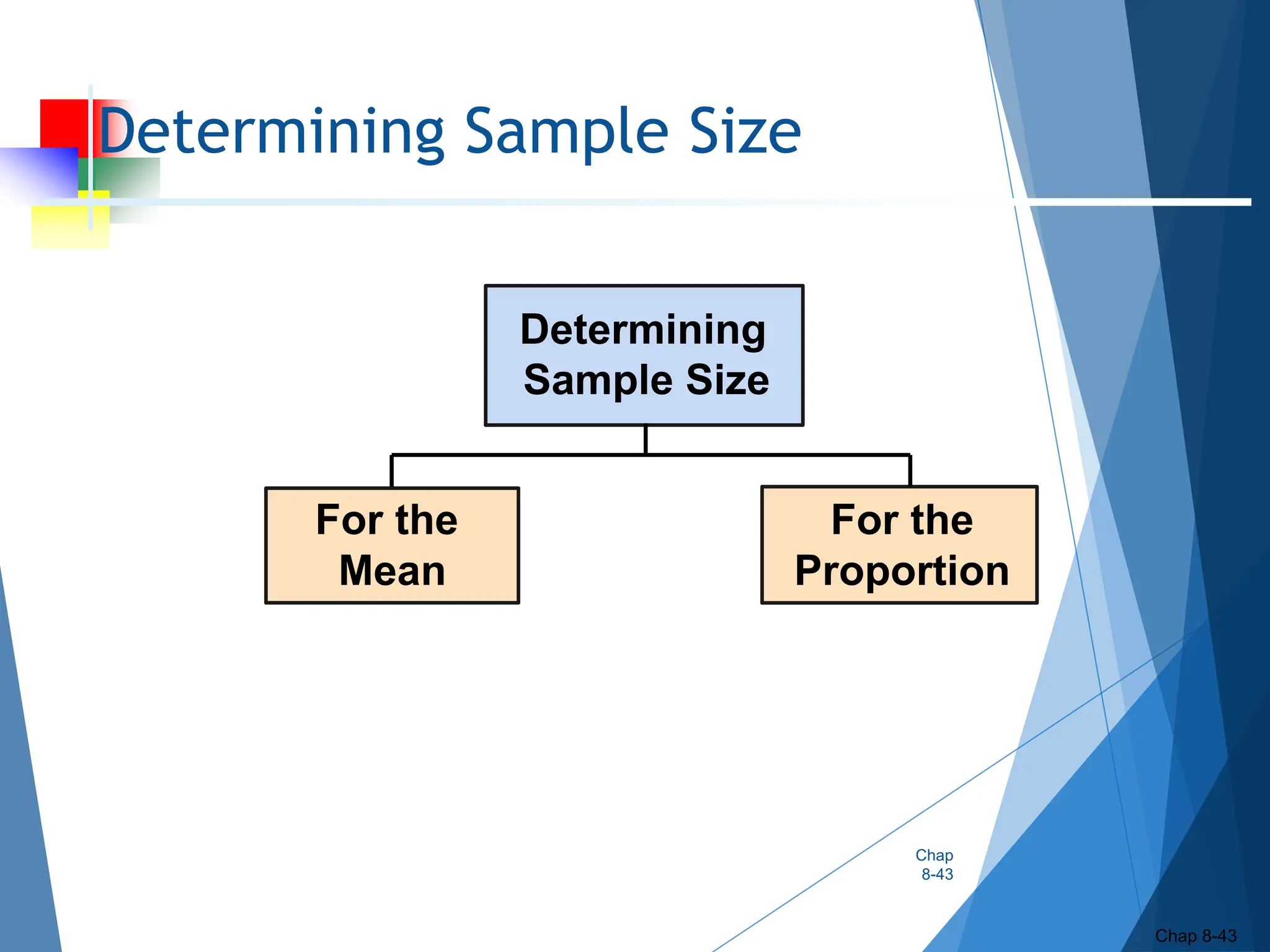
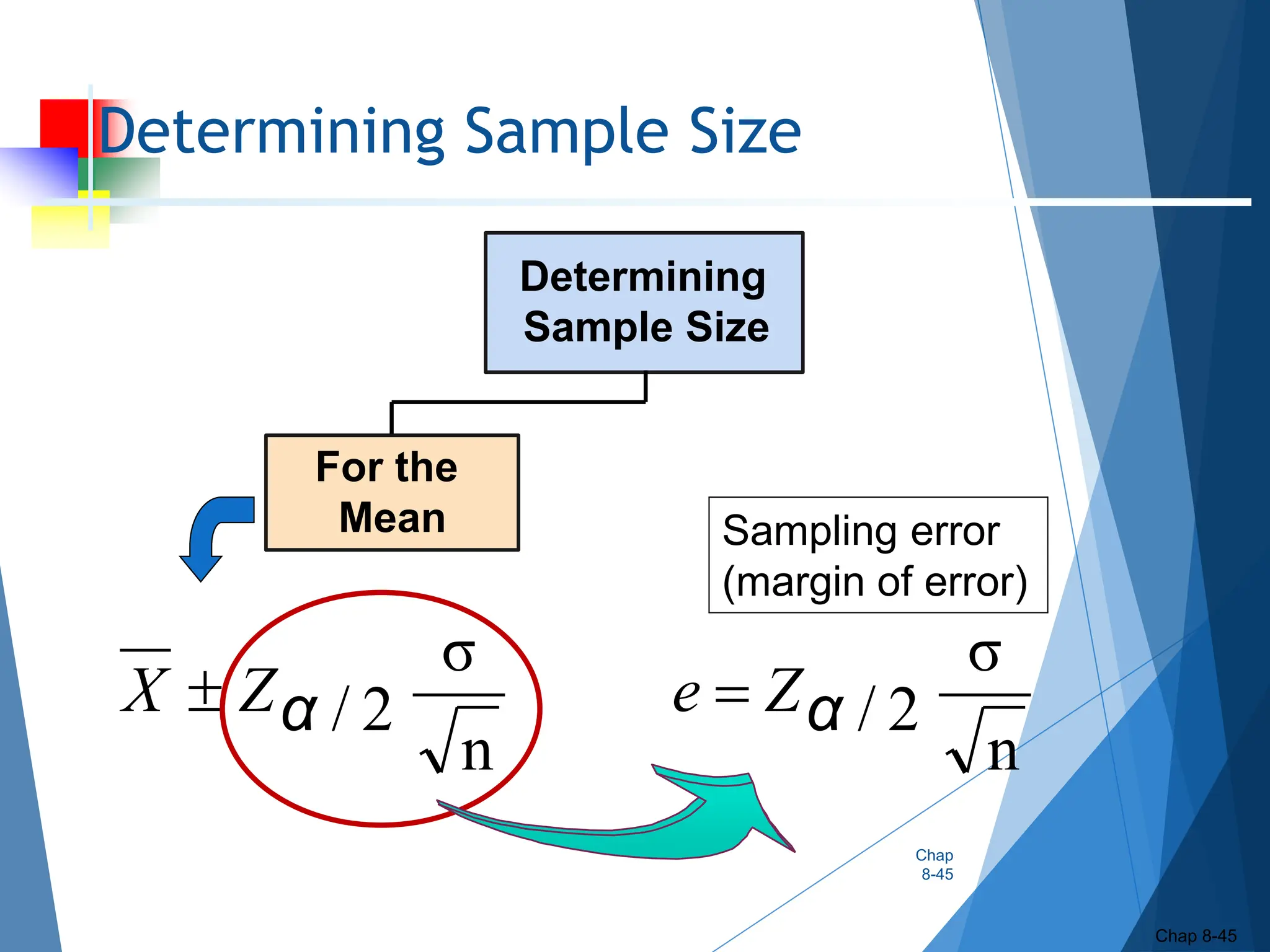
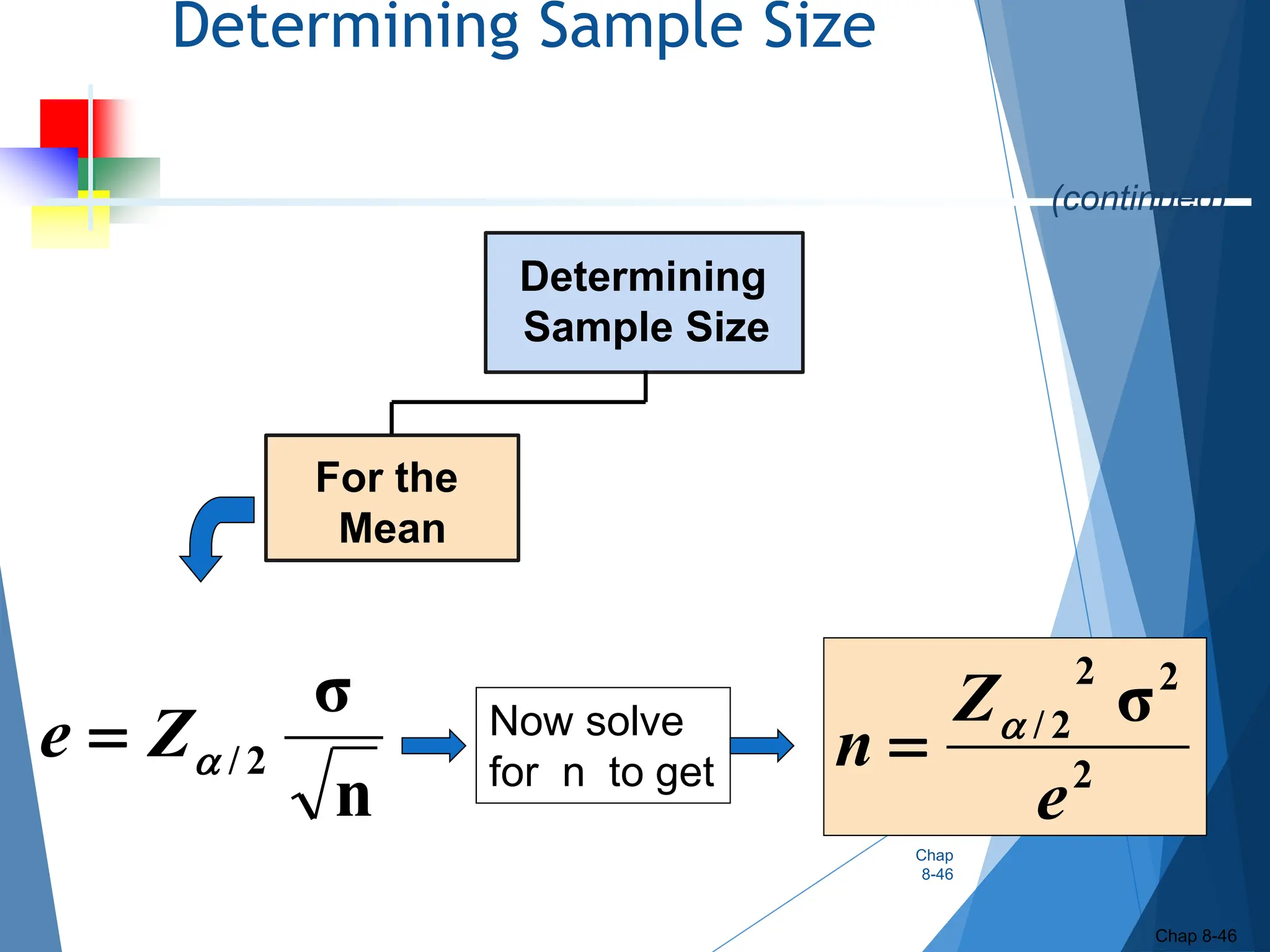
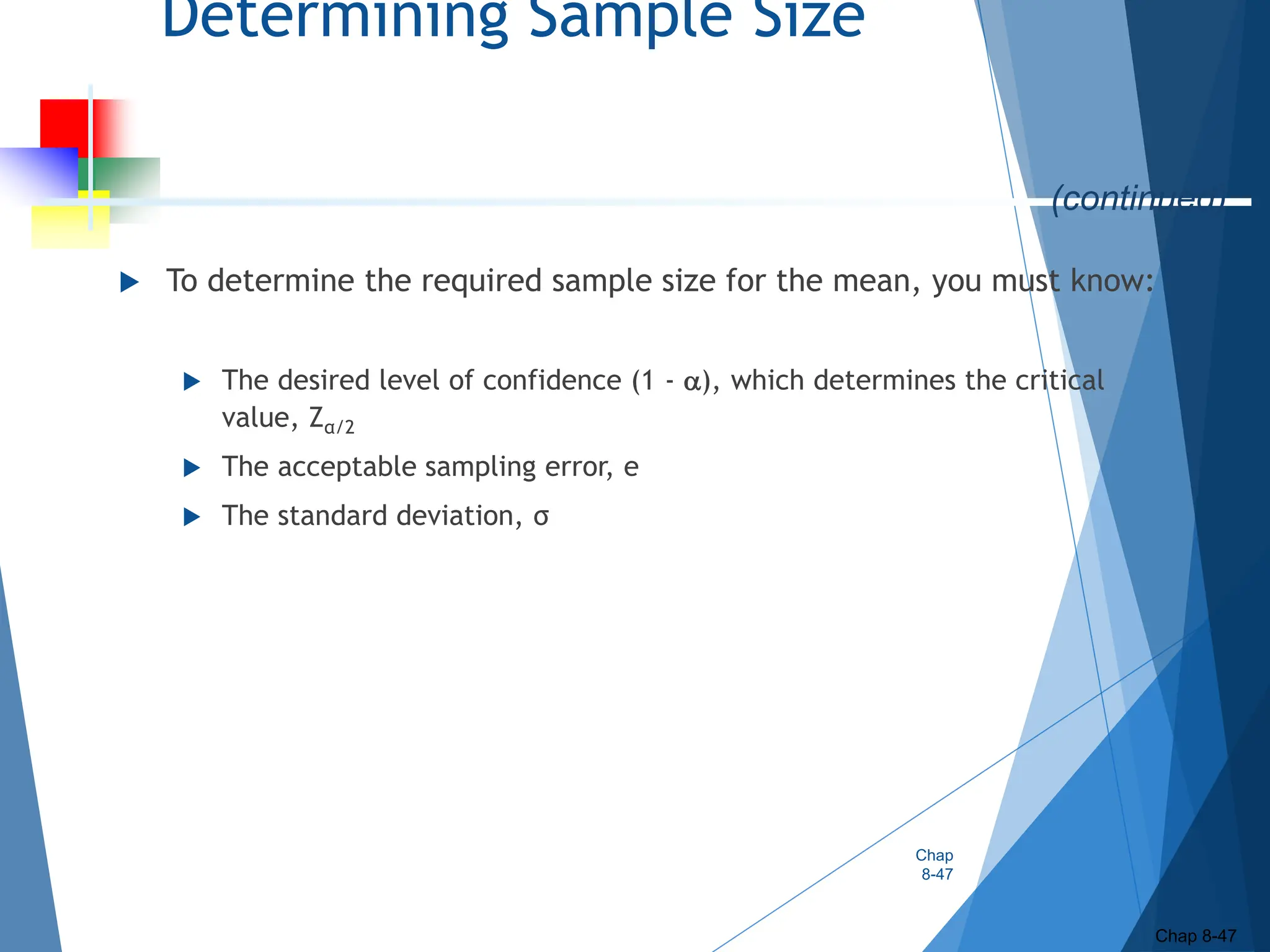
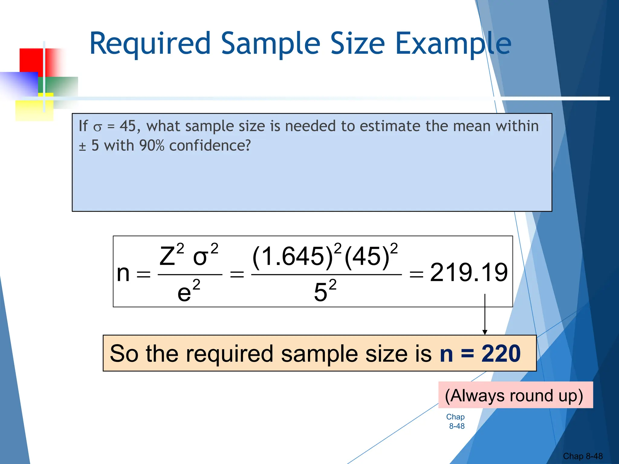
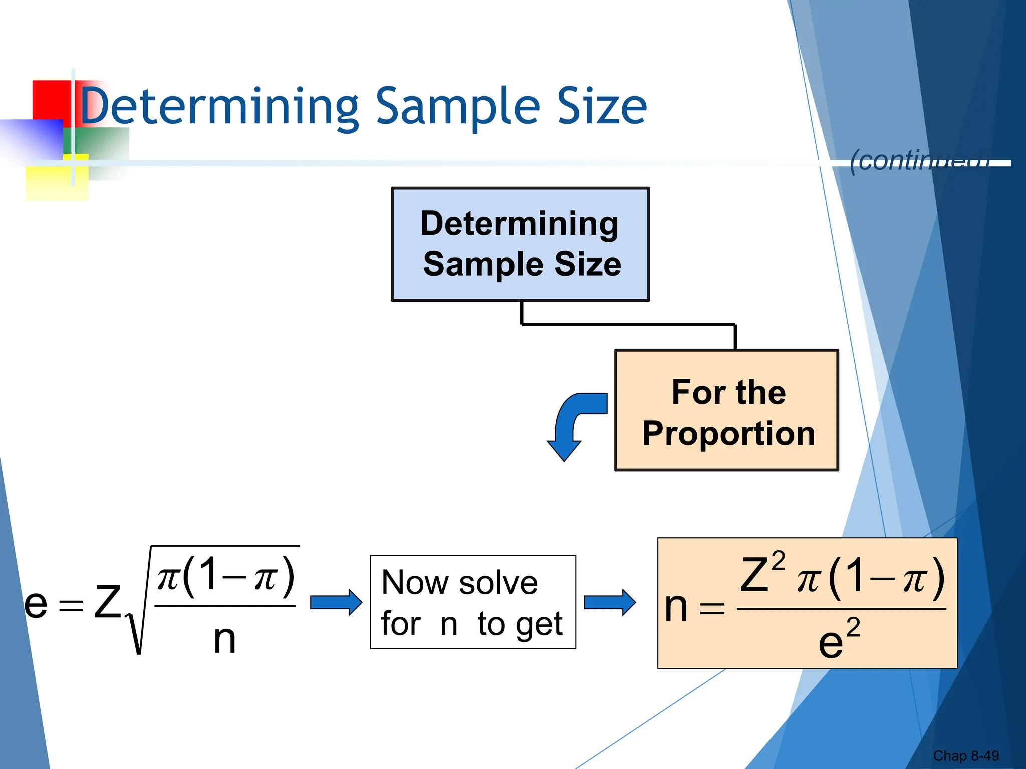
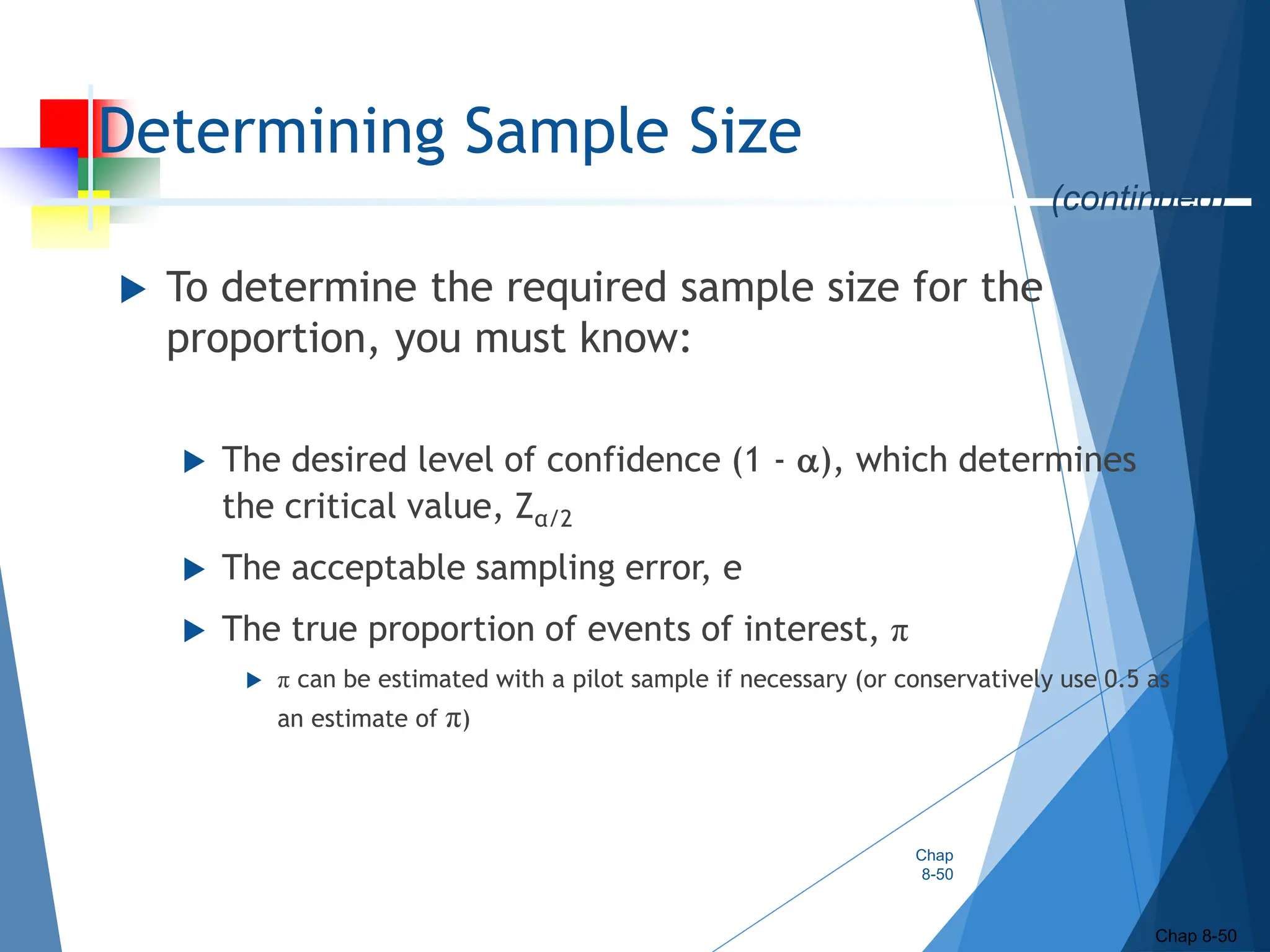
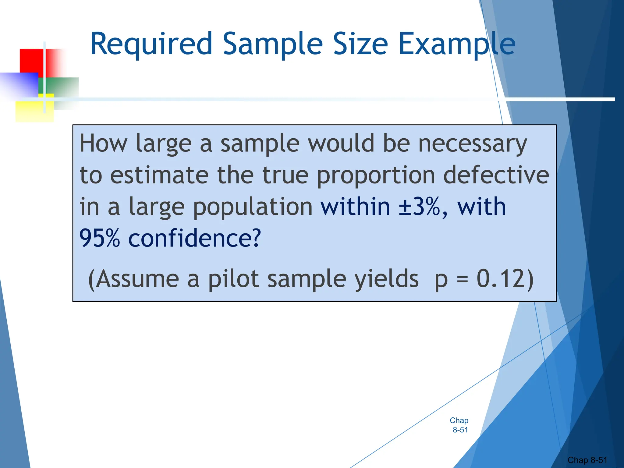
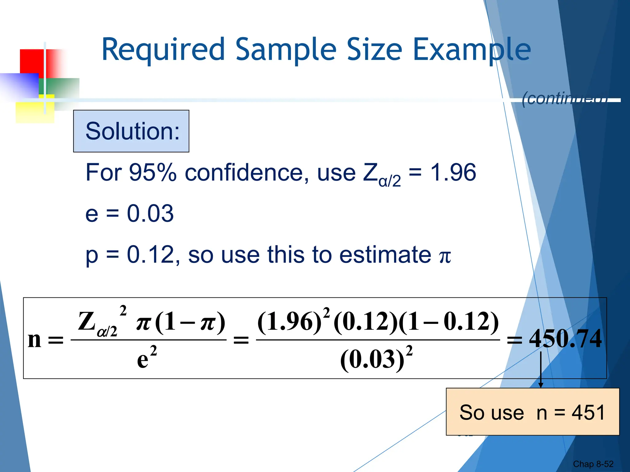

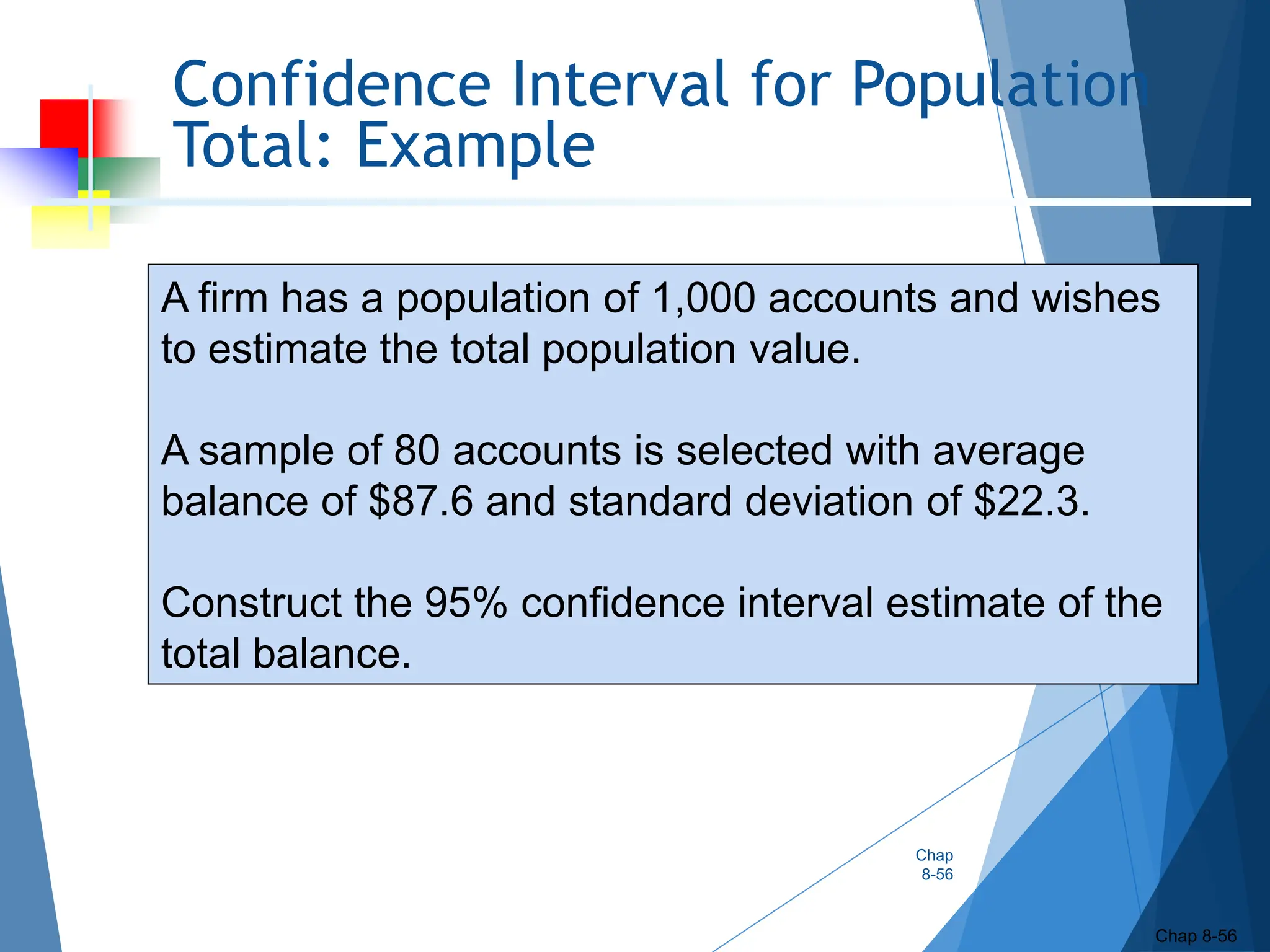
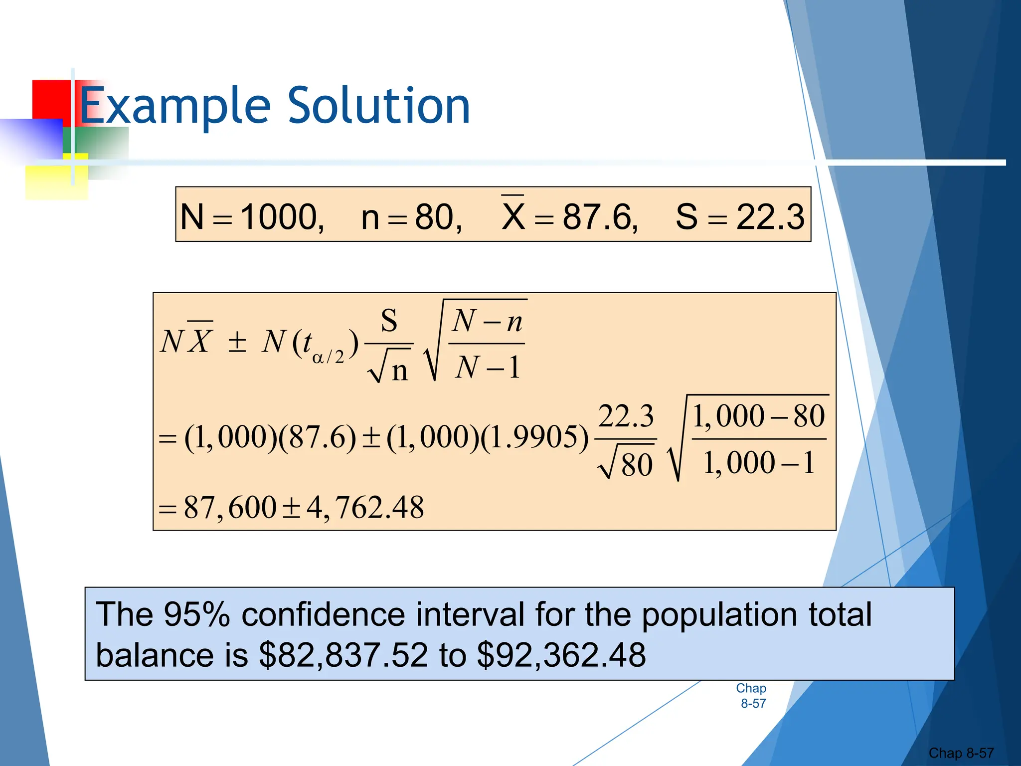
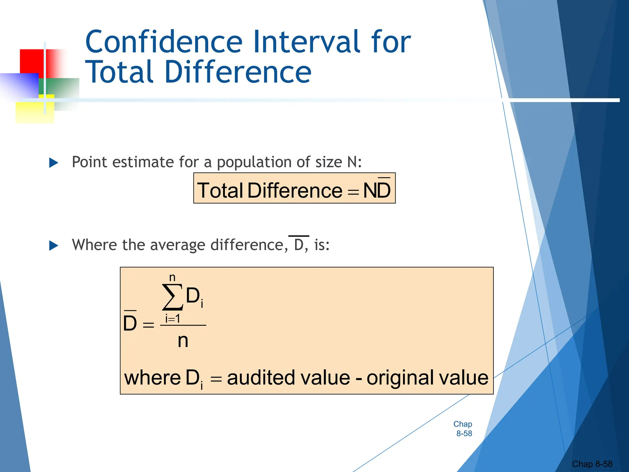
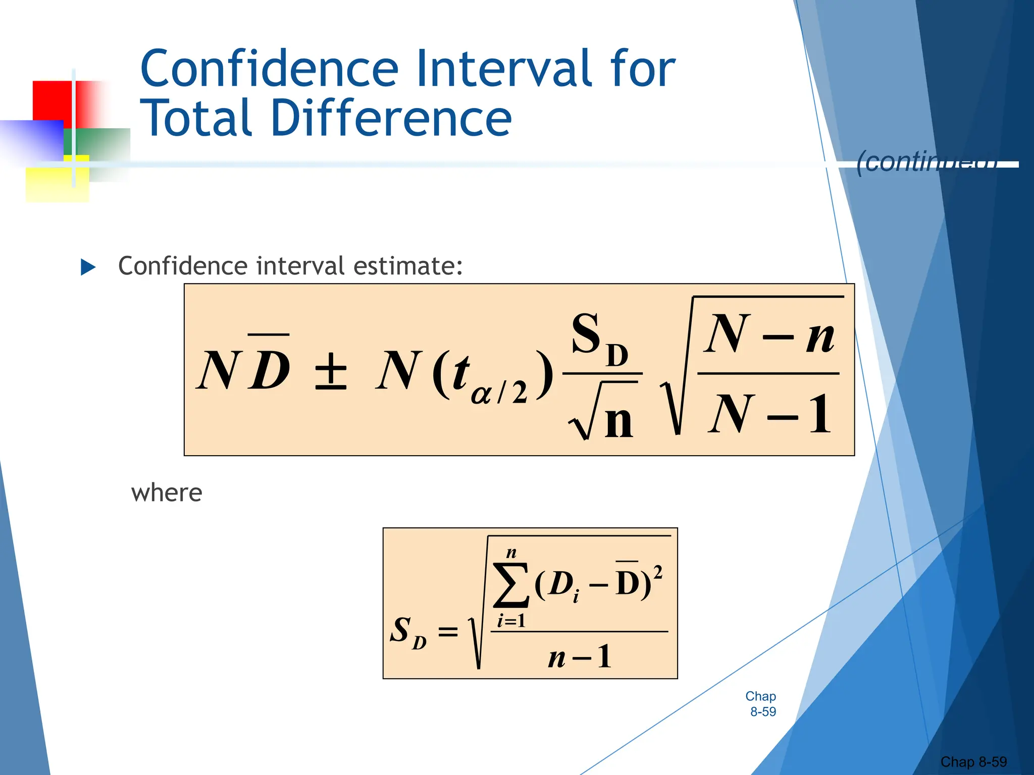
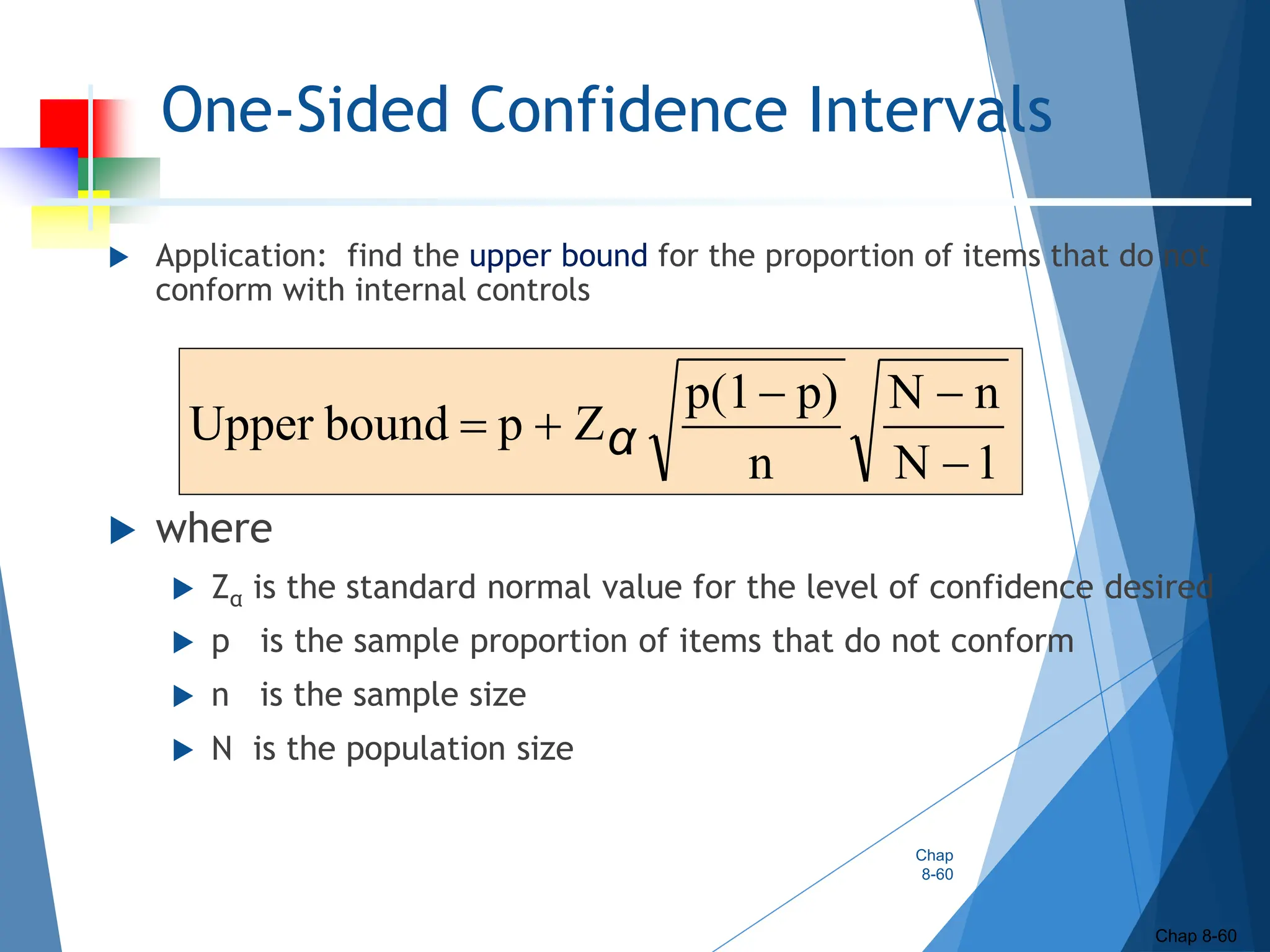
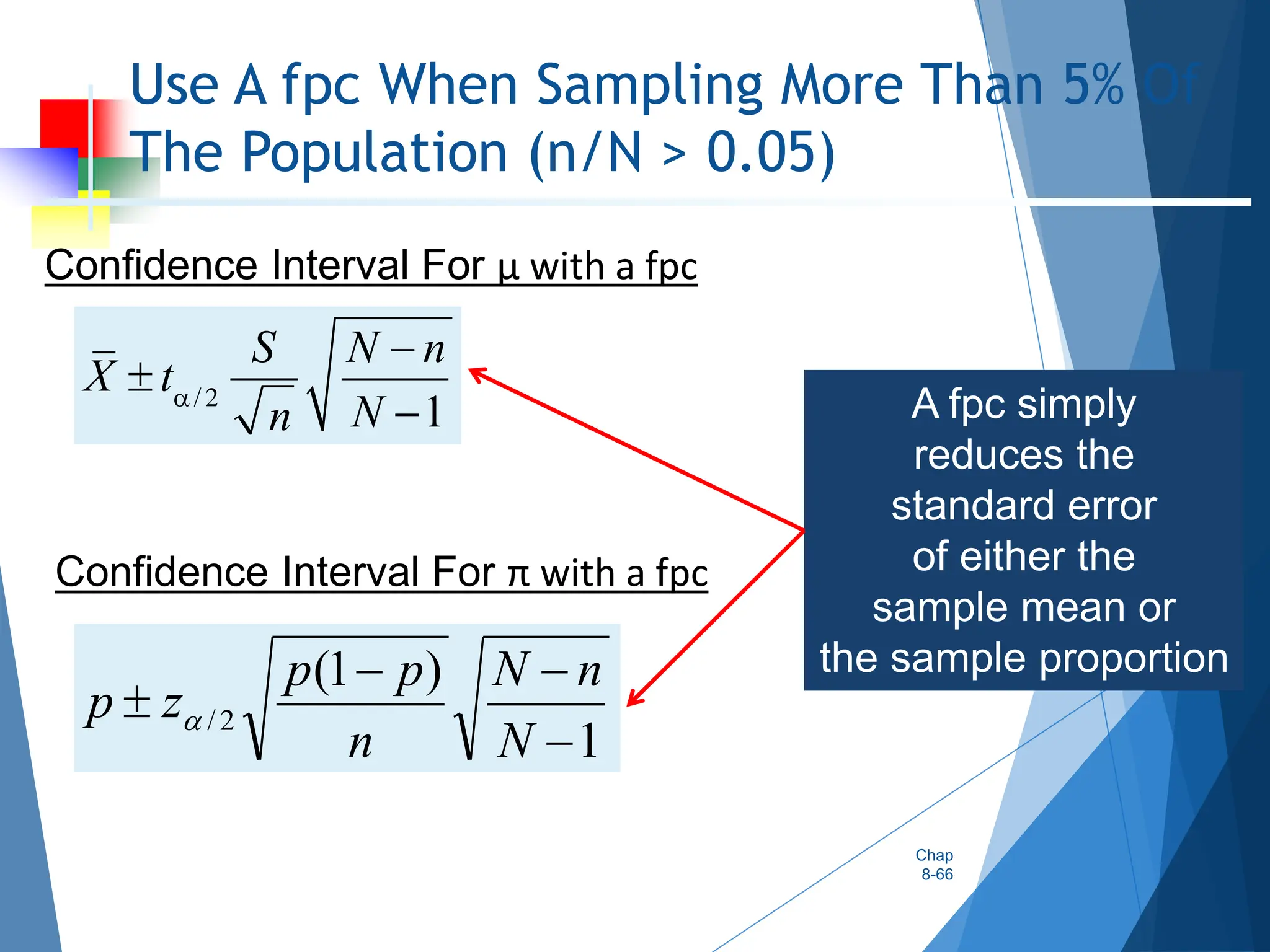
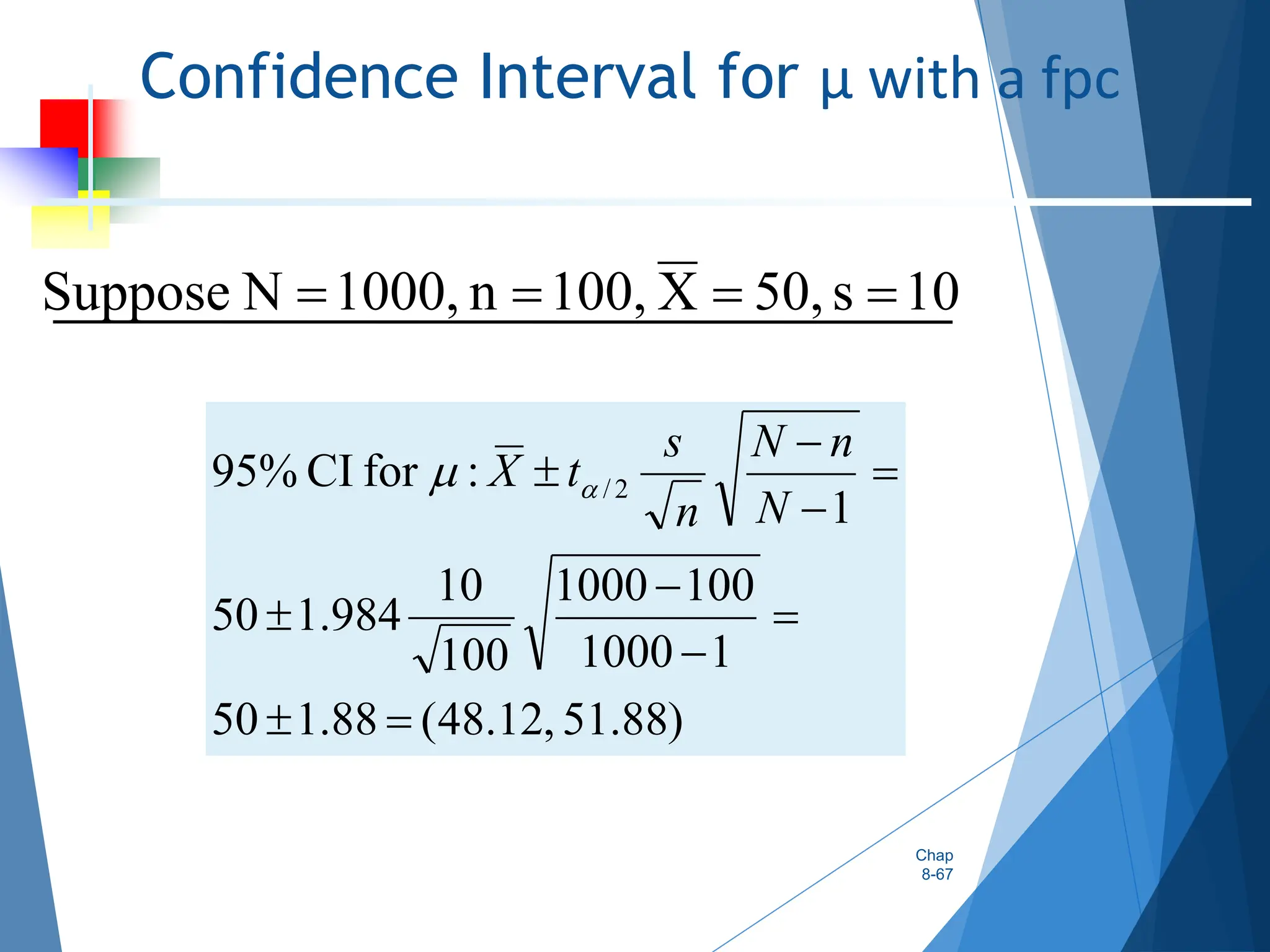
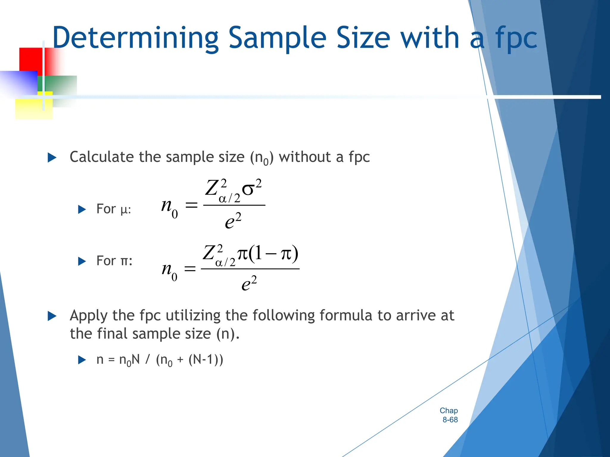

This document outlines key concepts related to constructing confidence intervals for estimating population means and proportions. It discusses how to calculate confidence intervals when the population standard deviation is known or unknown. Specifically, it provides the formulas and assumptions for constructing confidence intervals for a population mean using the normal and t-distributions. It also outlines how to calculate confidence intervals for a population proportion using the normal approximation. Examples are provided to demonstrate how to construct 95% confidence intervals for a mean and proportion based on sample data.


![[DSC Europe 25] Velibor Ilic - Autonomous Driving - How AI Shapes Technical ...](https://cdn.slidesharecdn.com/ss_thumbnails/gwu9aqths9ovngsrhidc-3-velibor-ilic-autonomous-driving-how-ai-shapes-technical-challenges-251219150035-7436923a-thumbnail.jpg?width=640&height=640&fit=bounds)
![[DSC Europe 25] Marko Djordjevic - AI can help Agriculture.pptx](https://cdn.slidesharecdn.com/ss_thumbnails/c0huq0ztiubmgccem2hc-marko-djordjevic-ai-can-help-agriculture-251218125253-7606f036-thumbnail.jpg?width=640&height=640&fit=bounds)


![[DSC Europe 25] Tatevik Maytesyan - How to actually use AI in marketing: gett...](https://cdn.slidesharecdn.com/ss_thumbnails/tjo626lsqdgfntbgl2mw-4-251216103155-e36cd239-thumbnail.jpg?width=640&height=640&fit=bounds)
![[DSC Europe 25] Jakub Stech - AI for Public Good: How Data and AI Can Transfo...](https://cdn.slidesharecdn.com/ss_thumbnails/ayuupcru6ggr9f7vbp0q-1-251215095918-7b7334a3-thumbnail.jpg?width=640&height=640&fit=bounds)
![[DSC Europe 25] Miodrag Pesovic & Vladislav Radonjic - Federated Data Archite...](https://cdn.slidesharecdn.com/ss_thumbnails/gsbe3y5it5uhndi4e08e-1-251212103249-f1008e0c-thumbnail.jpg?width=640&height=640&fit=bounds)
![[DSC Europe 25] Branko Urosevic -Rethinking Financial Talent: Integrating Cod...](https://cdn.slidesharecdn.com/ss_thumbnails/8jjrus8ttko6qj64f58f-3-251212103250-642c6374-thumbnail.jpg?width=640&height=640&fit=bounds)
![[DSC Europe 25] Debmalya Biswas - Agentification: the art of transforming man...](https://cdn.slidesharecdn.com/ss_thumbnails/r5azlggvtqiaiiusrqdr-4-251212103249-5a12c89b-thumbnail.jpg?width=640&height=640&fit=bounds)


![[DSC Europe 25] Katherine Forrest - AI NOW: Understanding the Velocity of Cha...](https://cdn.slidesharecdn.com/ss_thumbnails/wvvbruqfrci0sfq9xwgb-4-251212104007-e5ad1987-thumbnail.jpg?width=640&height=640&fit=bounds)