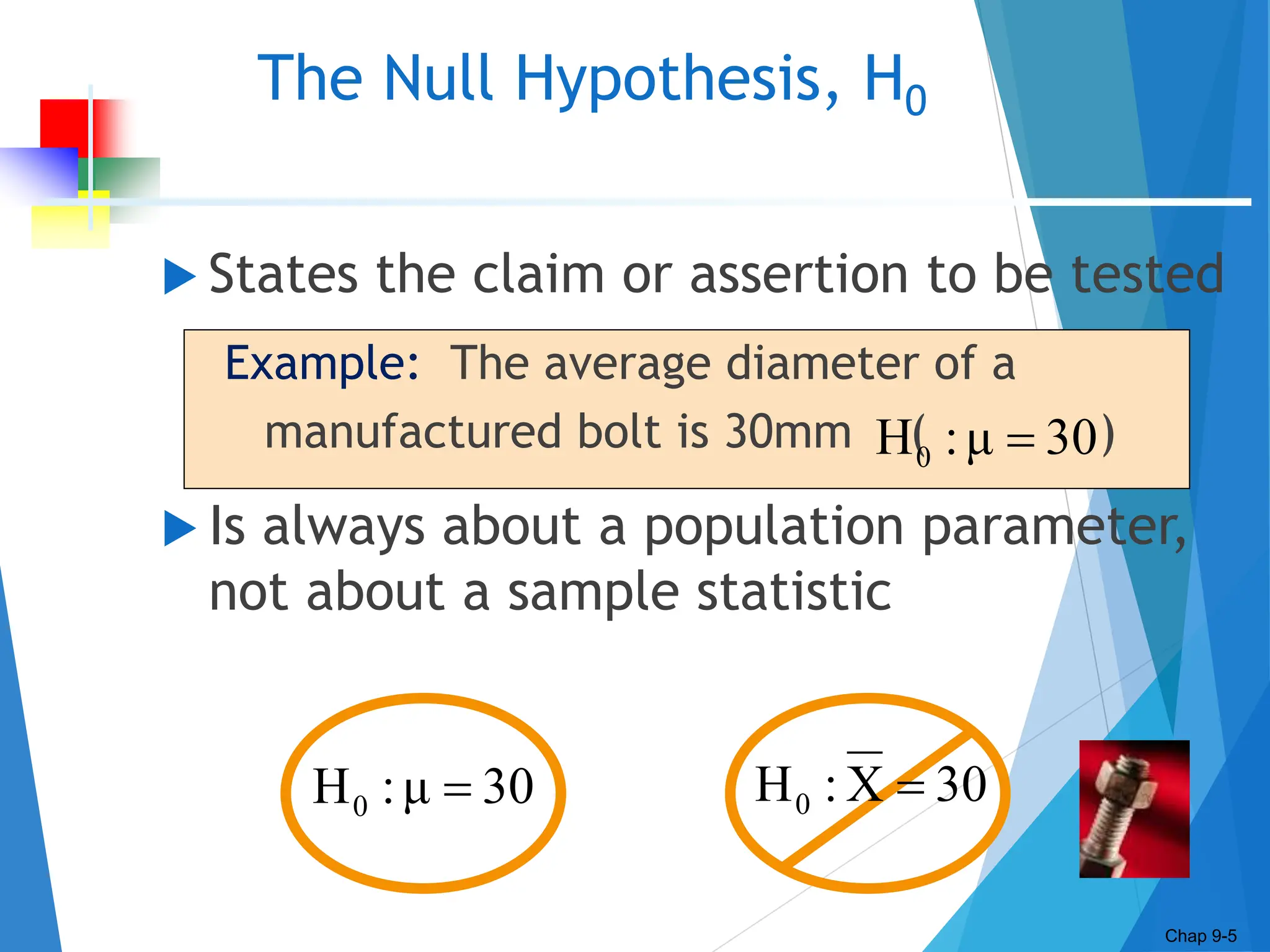
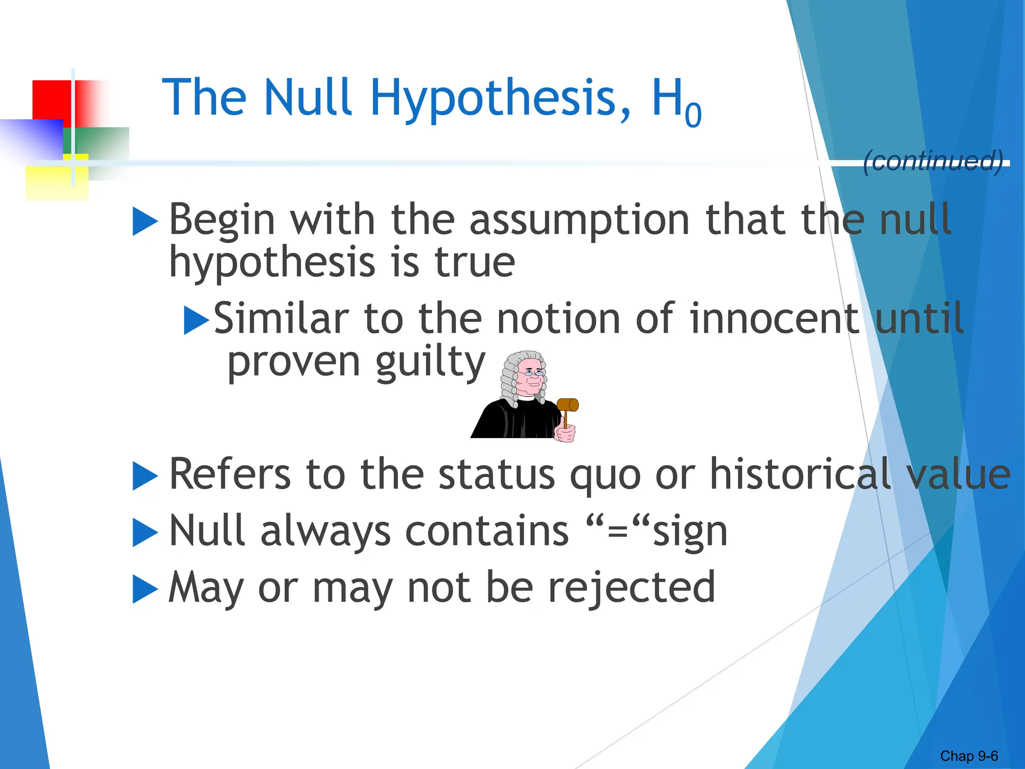
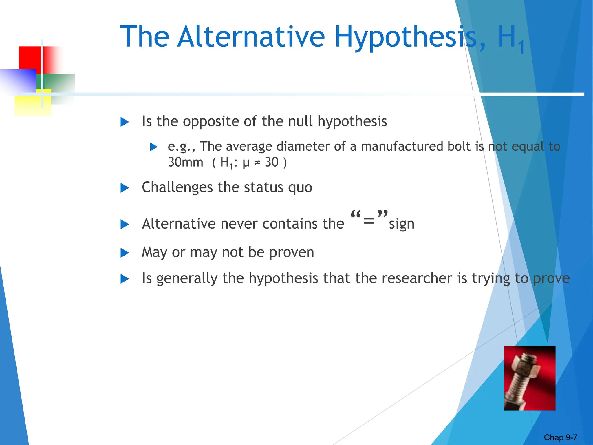
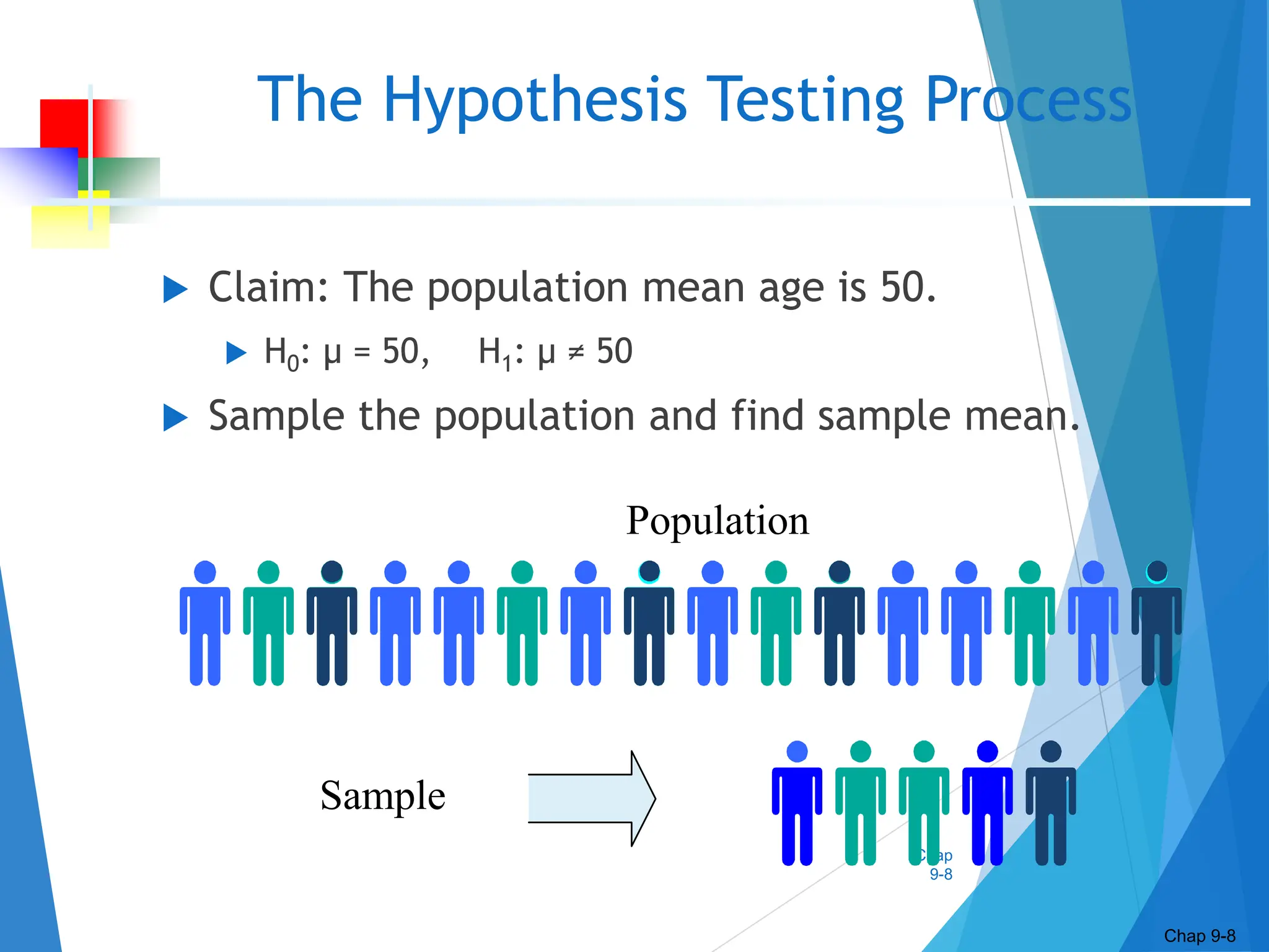
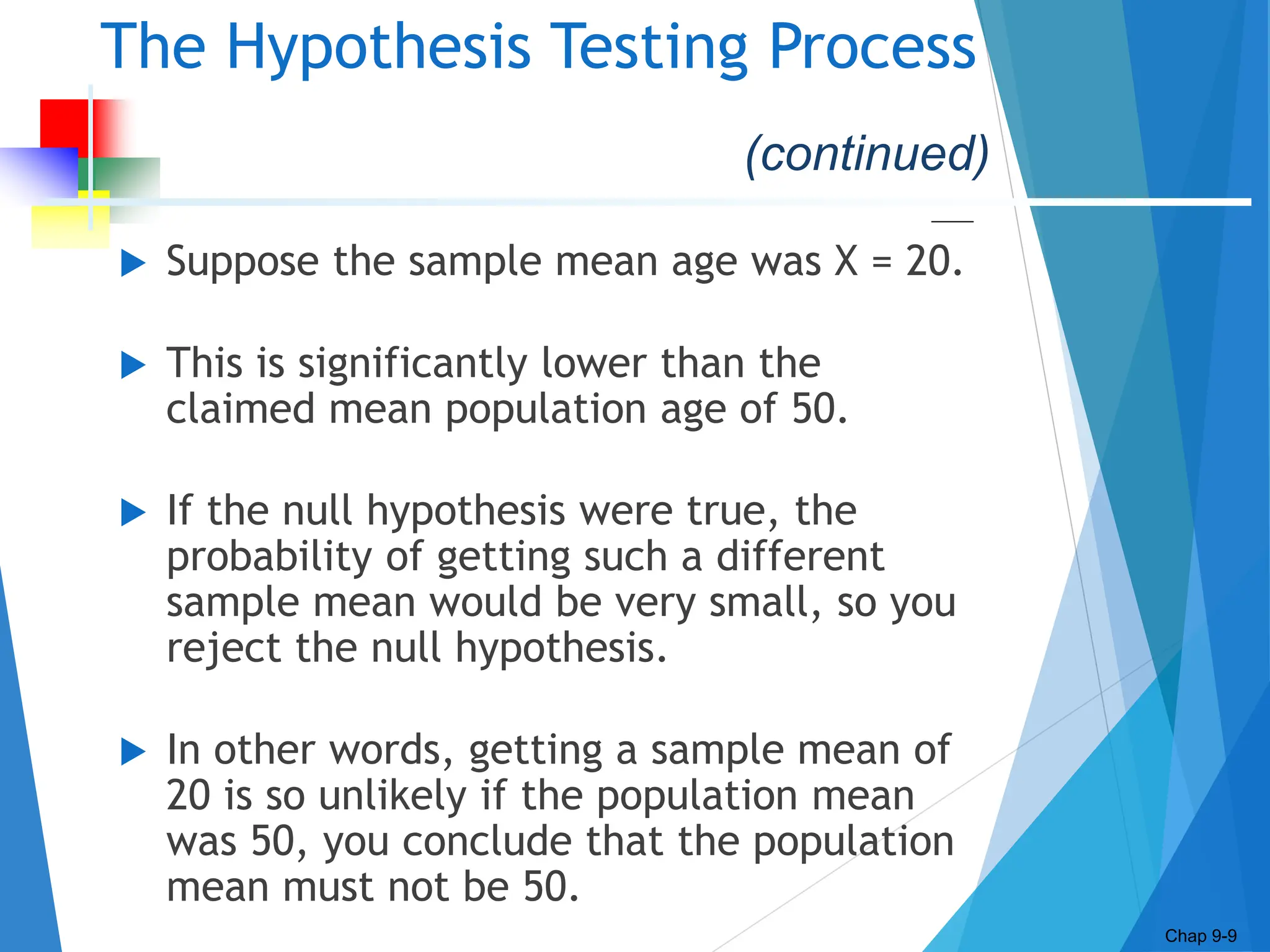
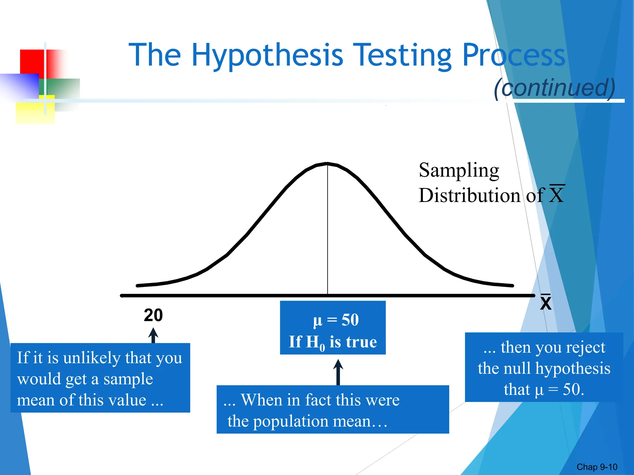
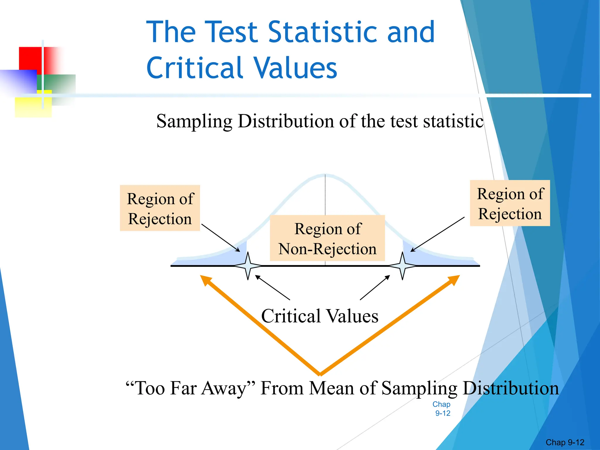
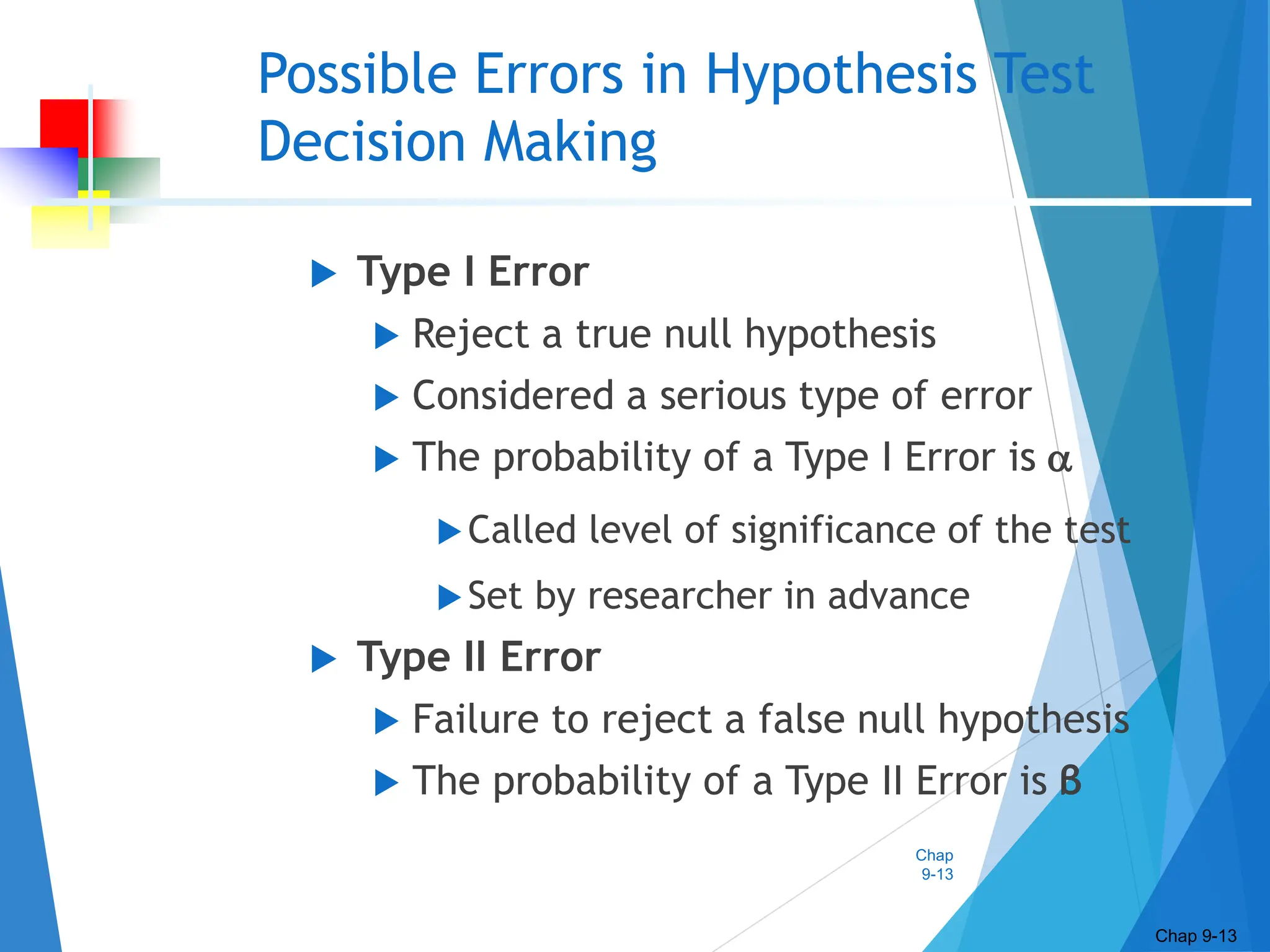
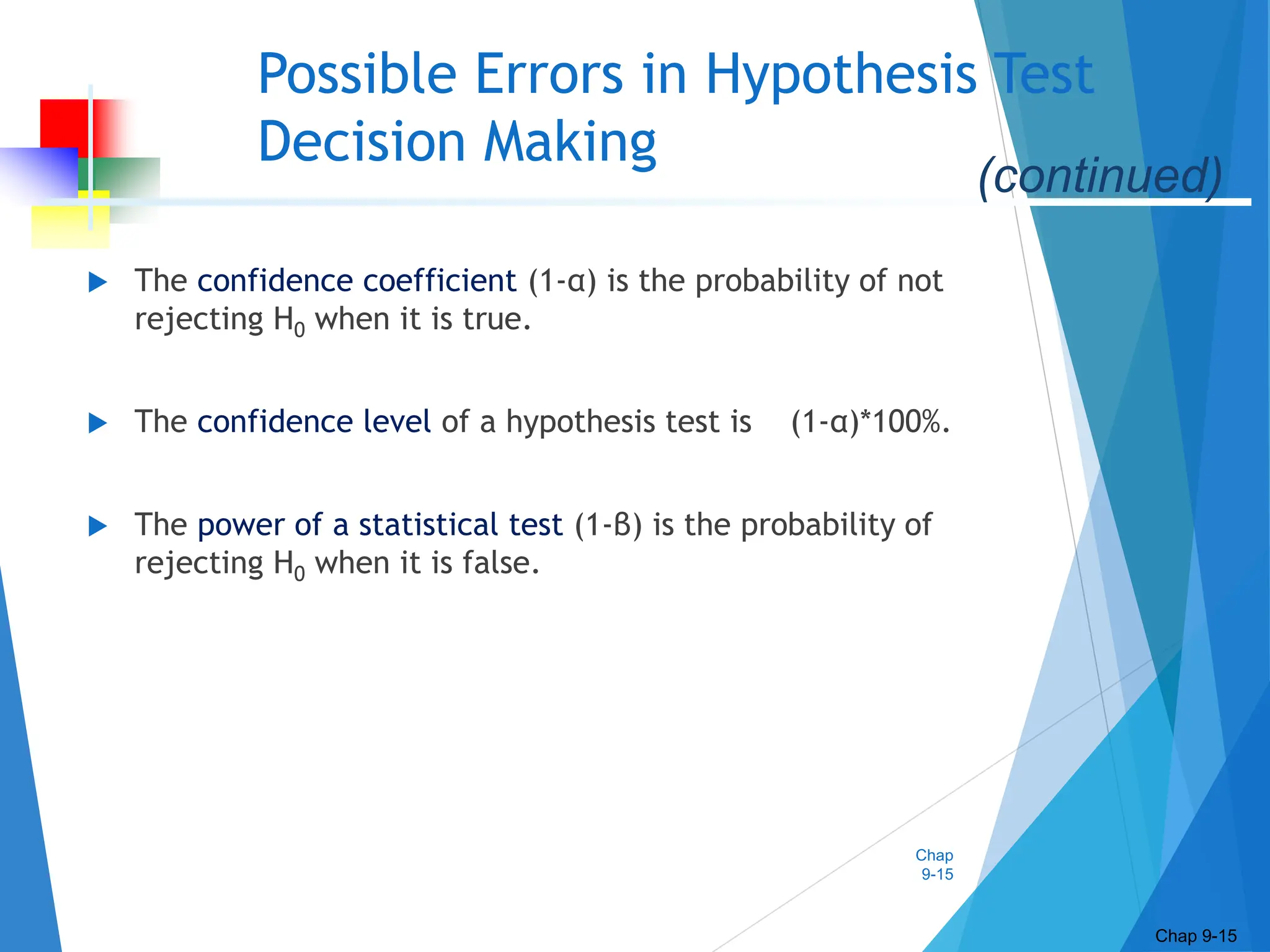
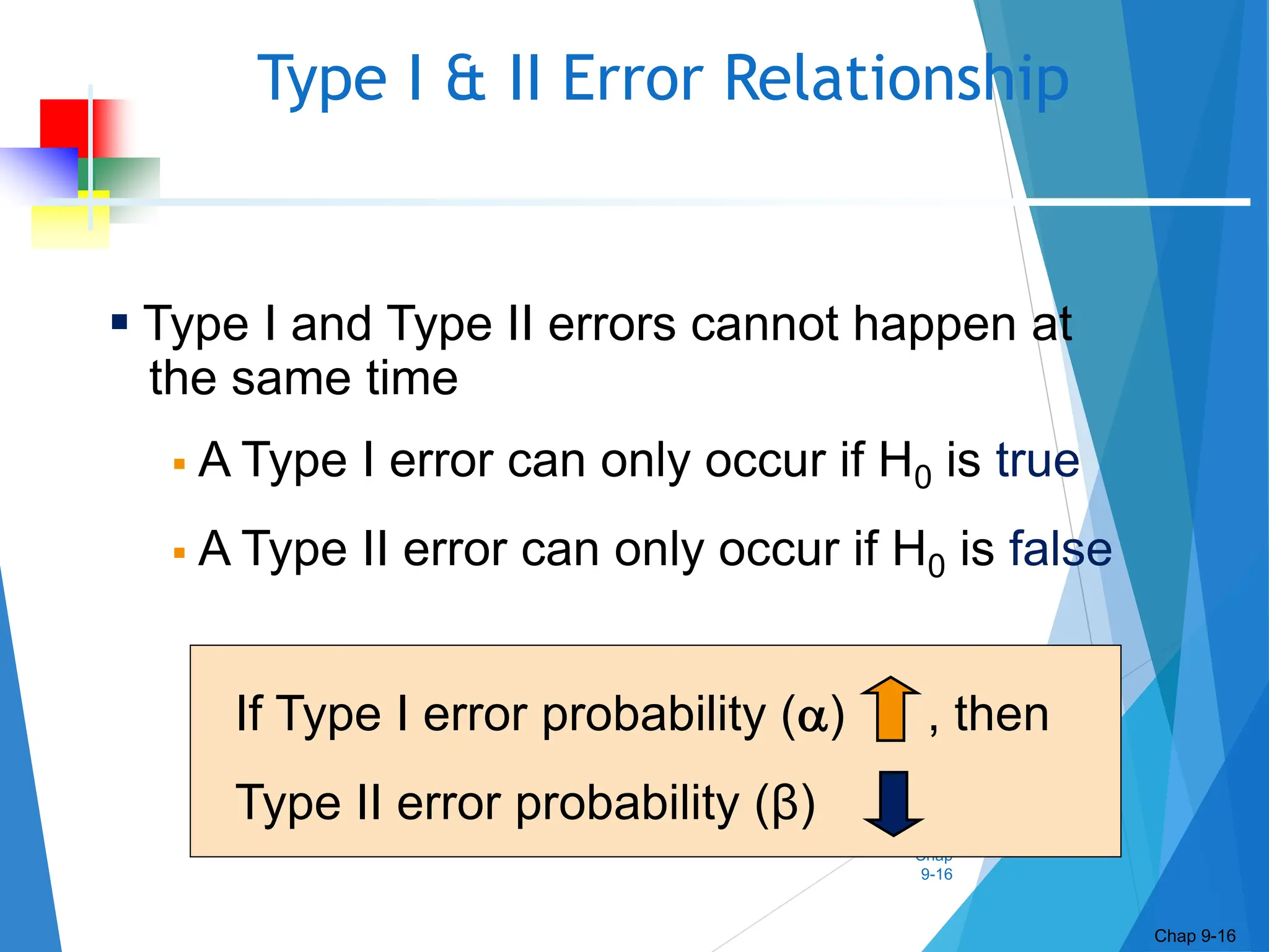
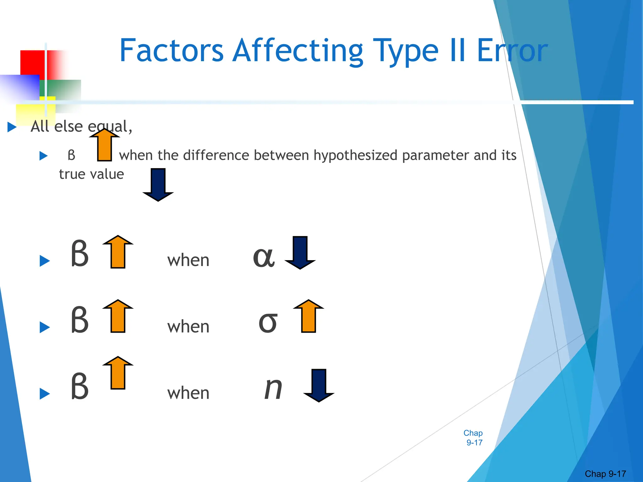
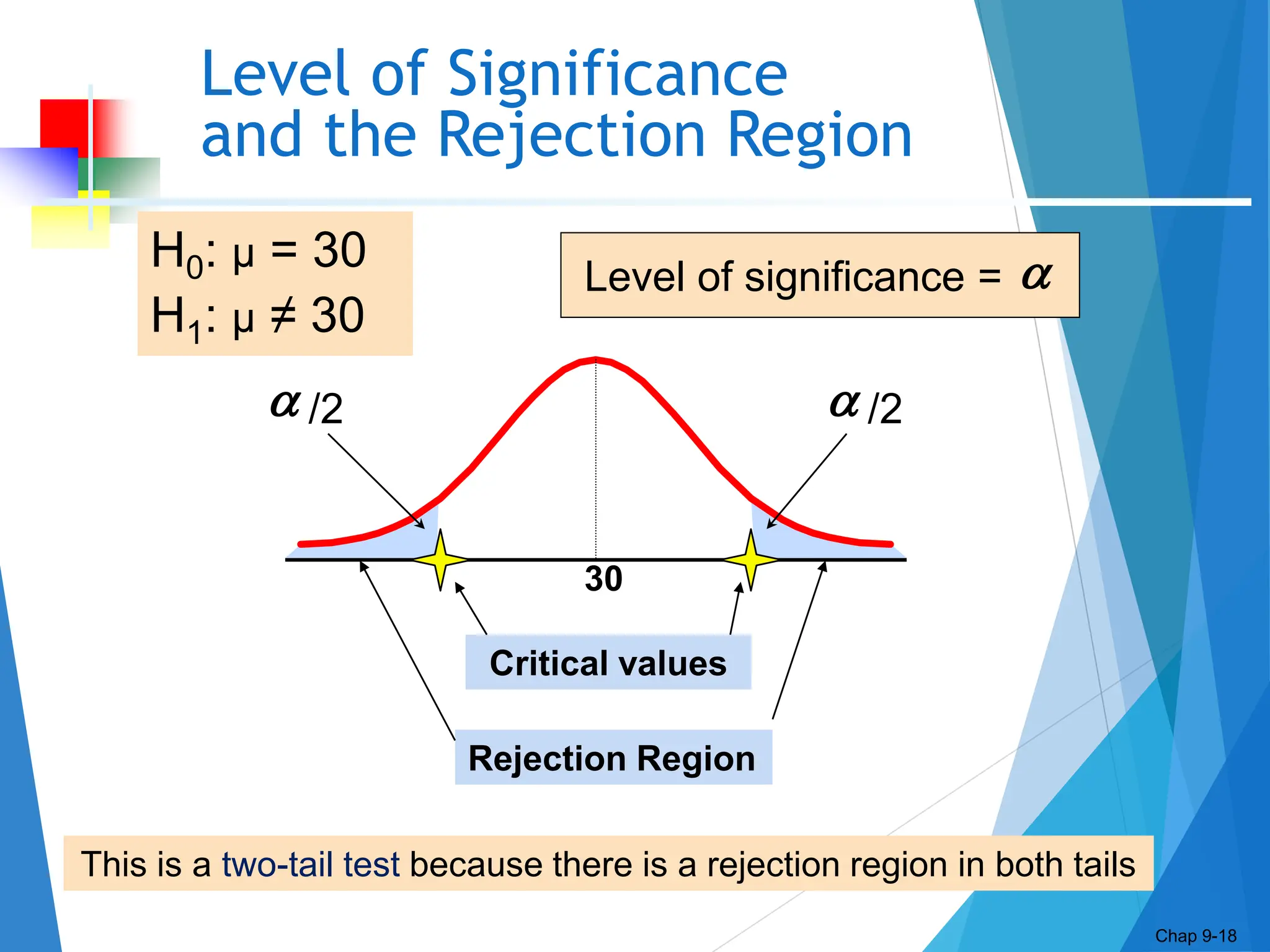
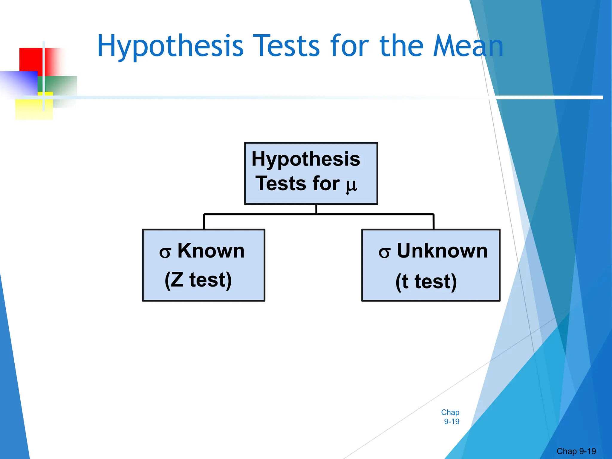
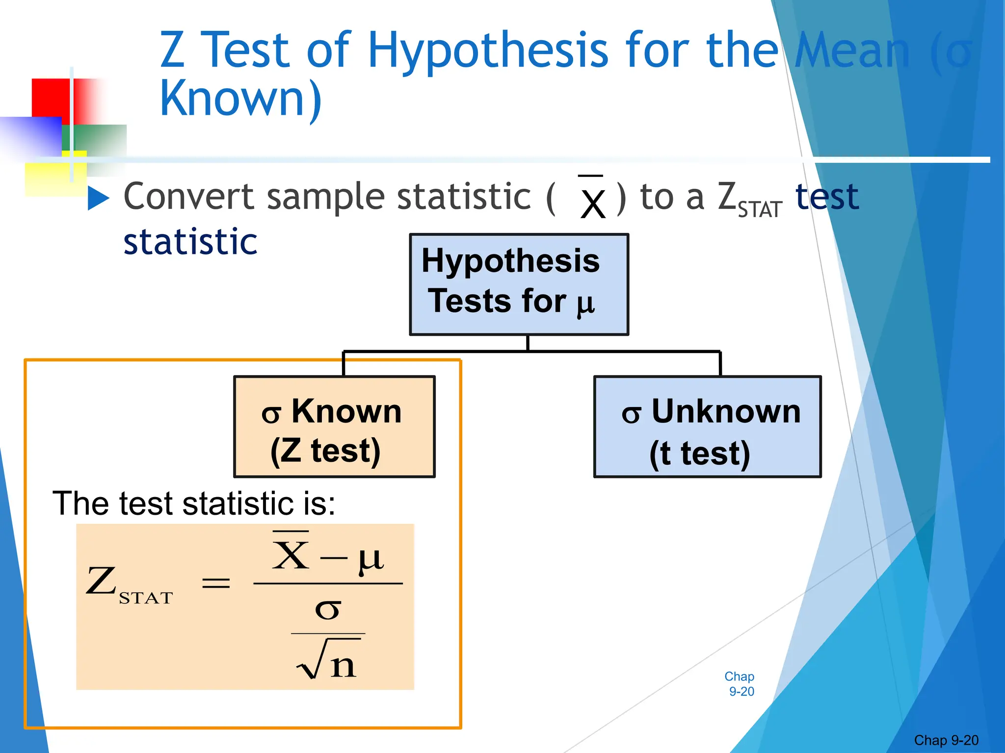
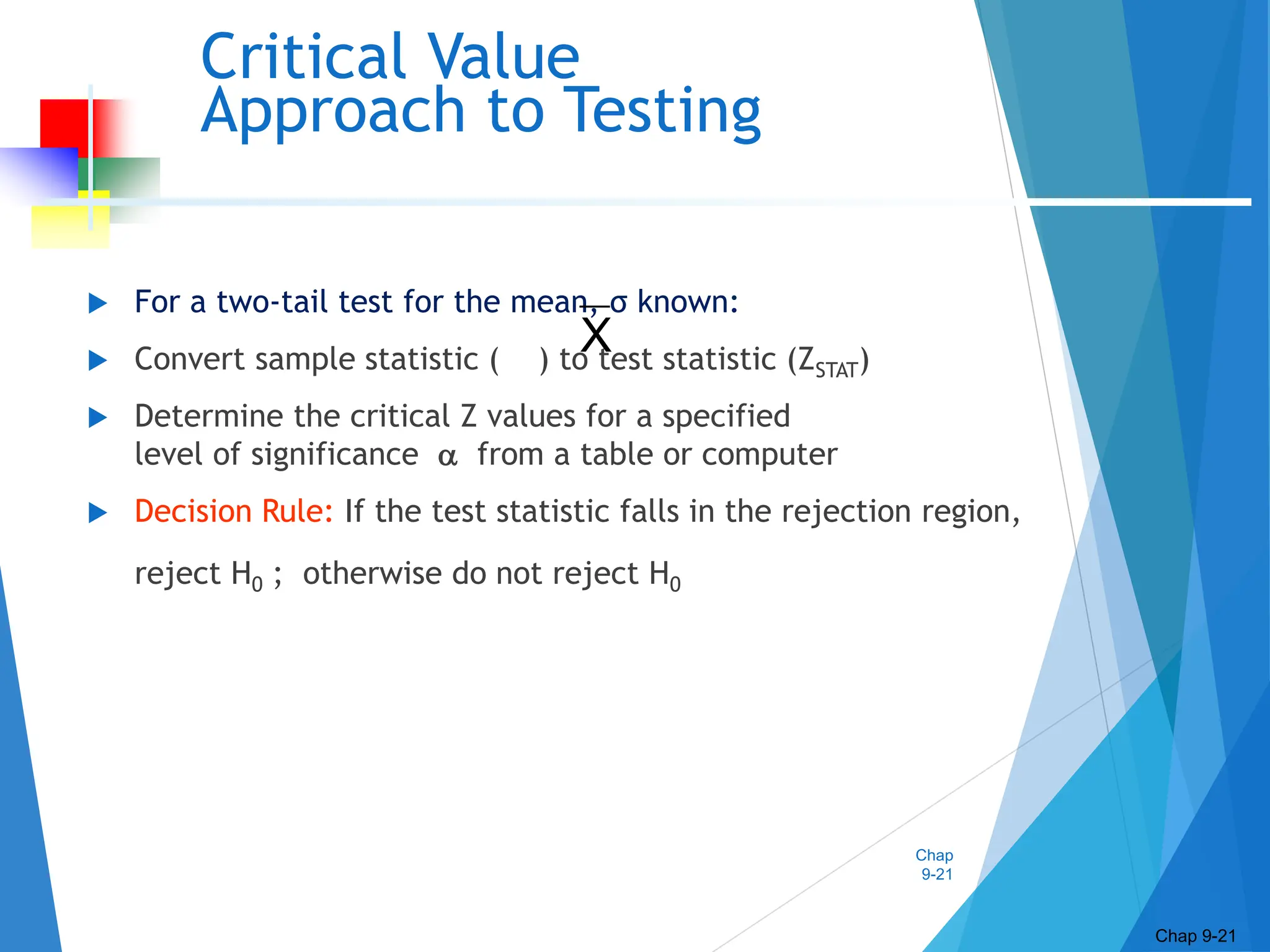
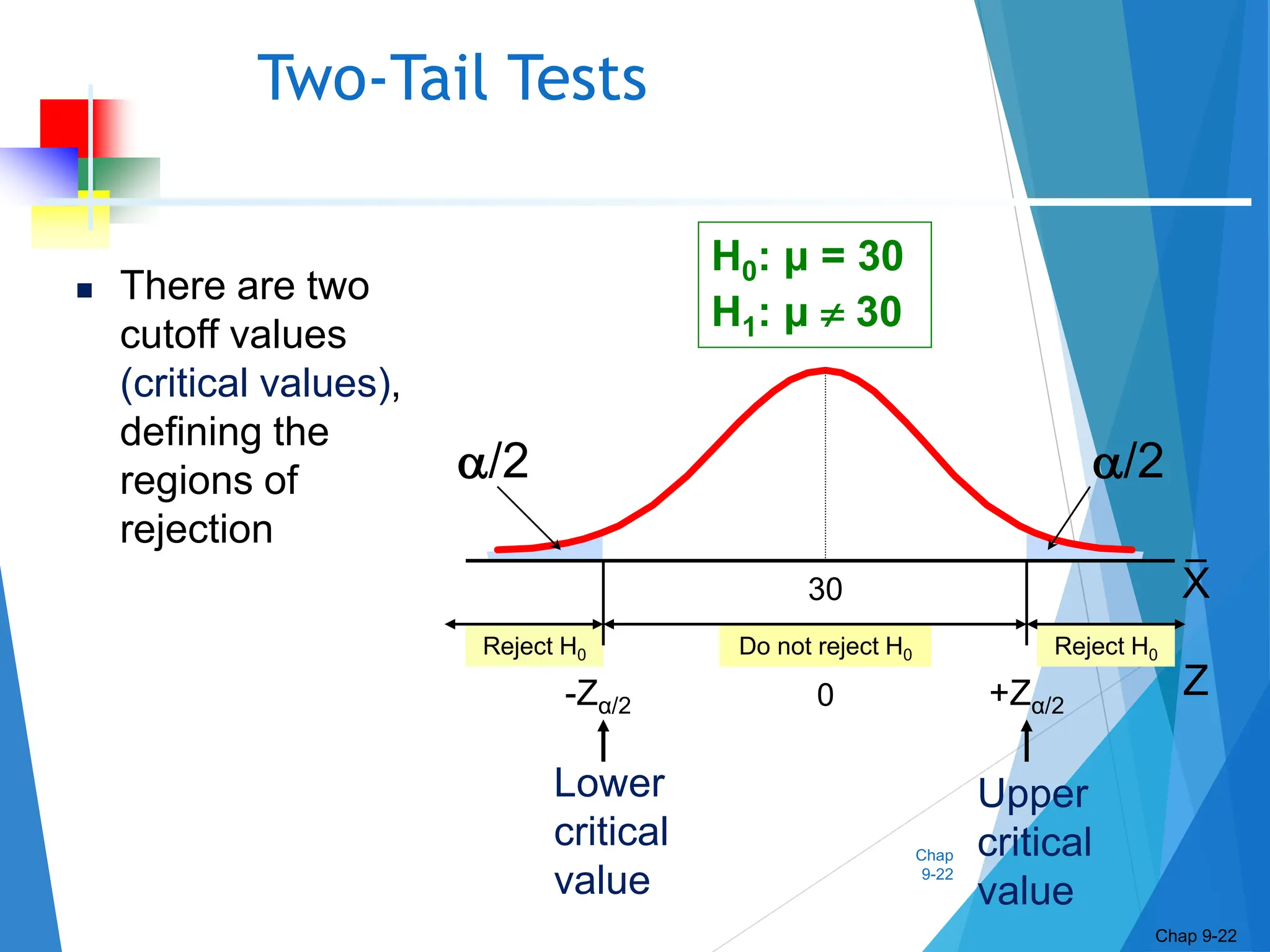
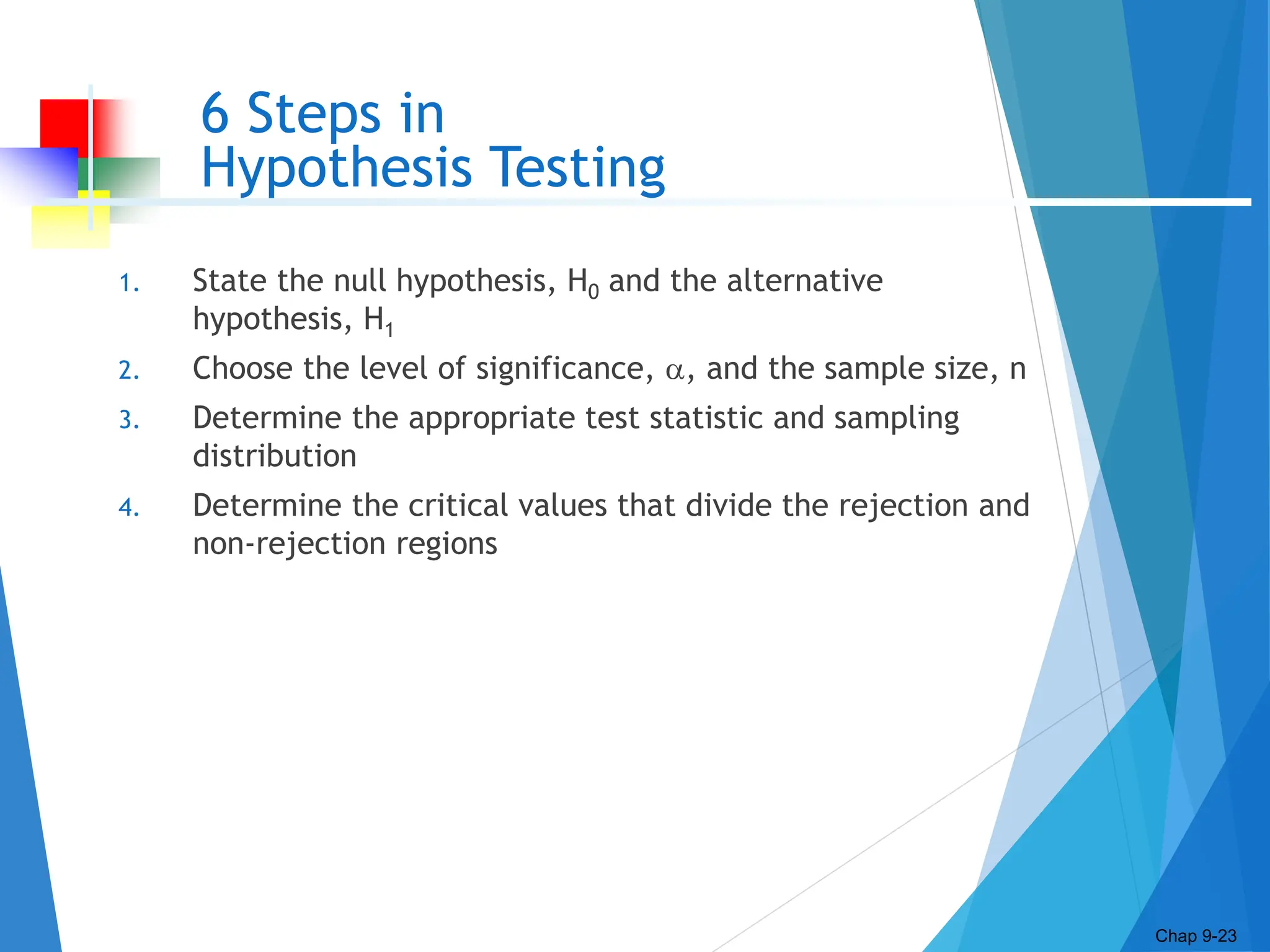
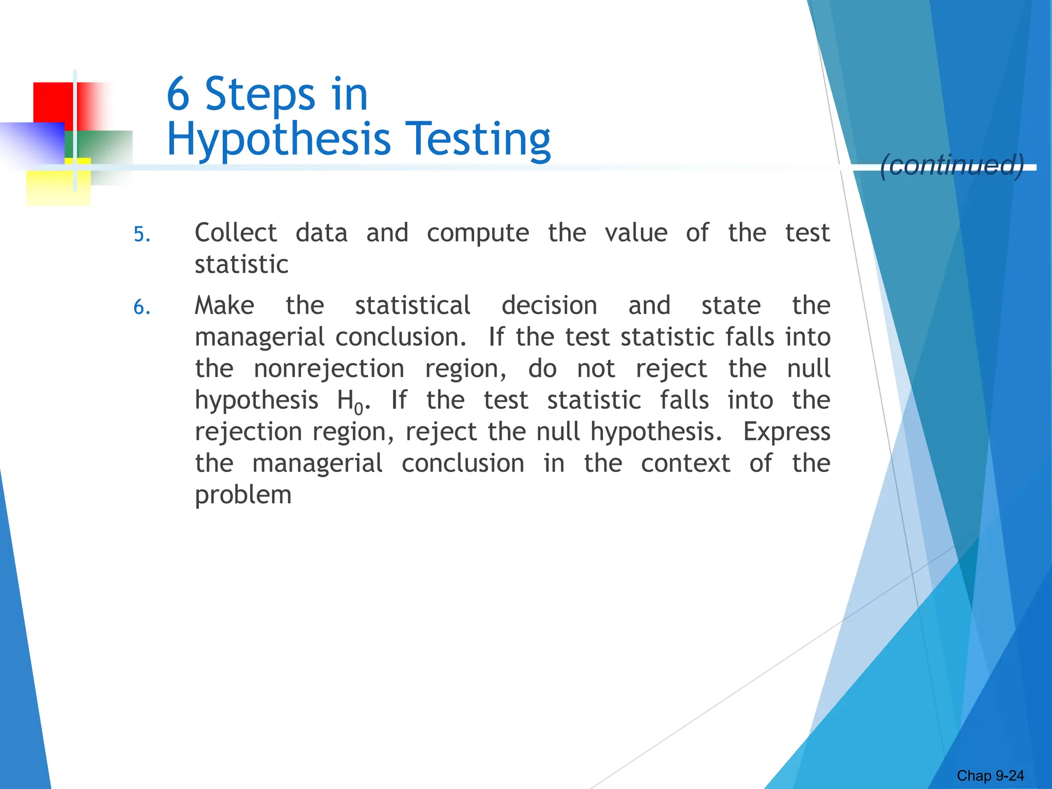
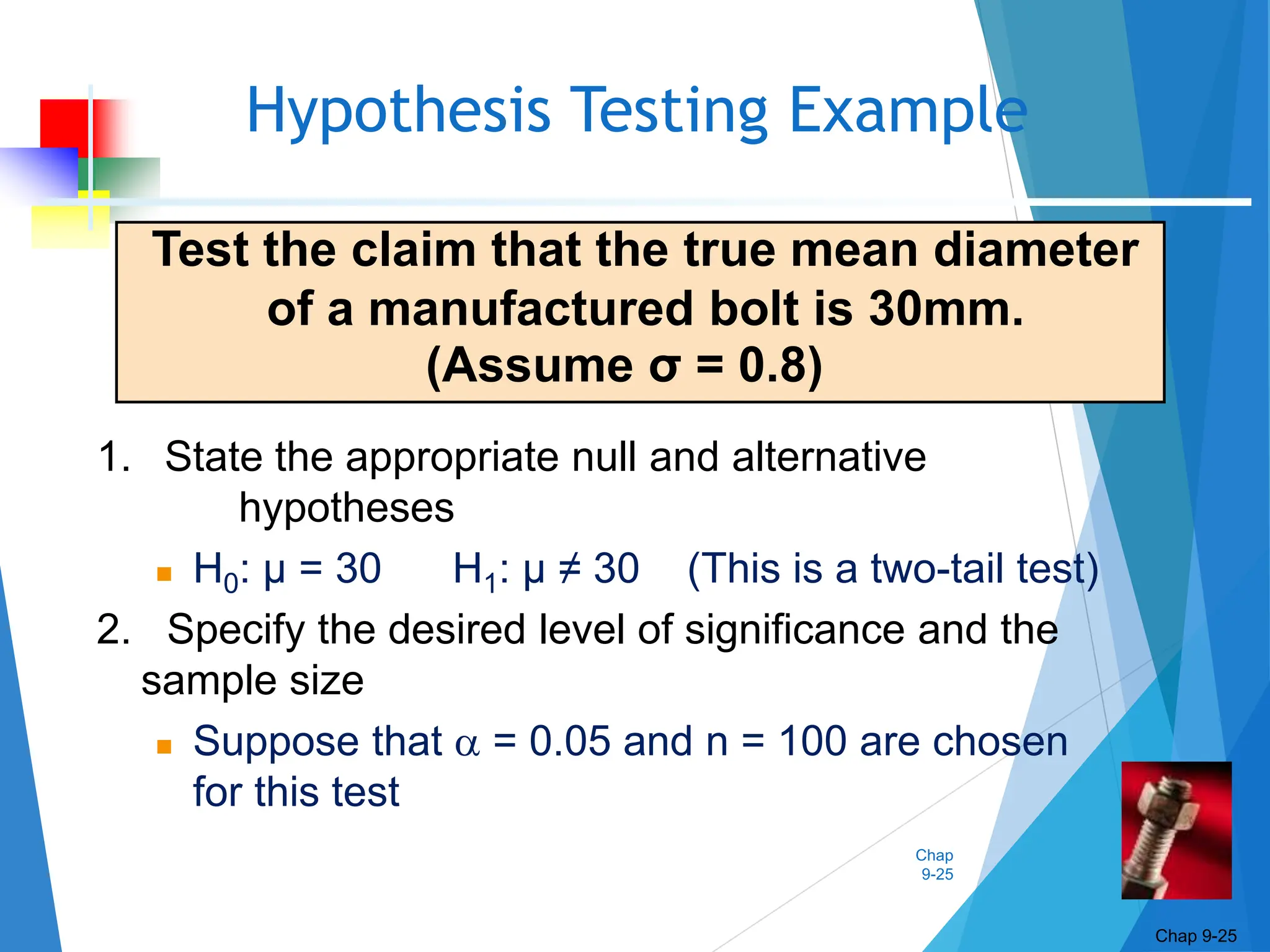
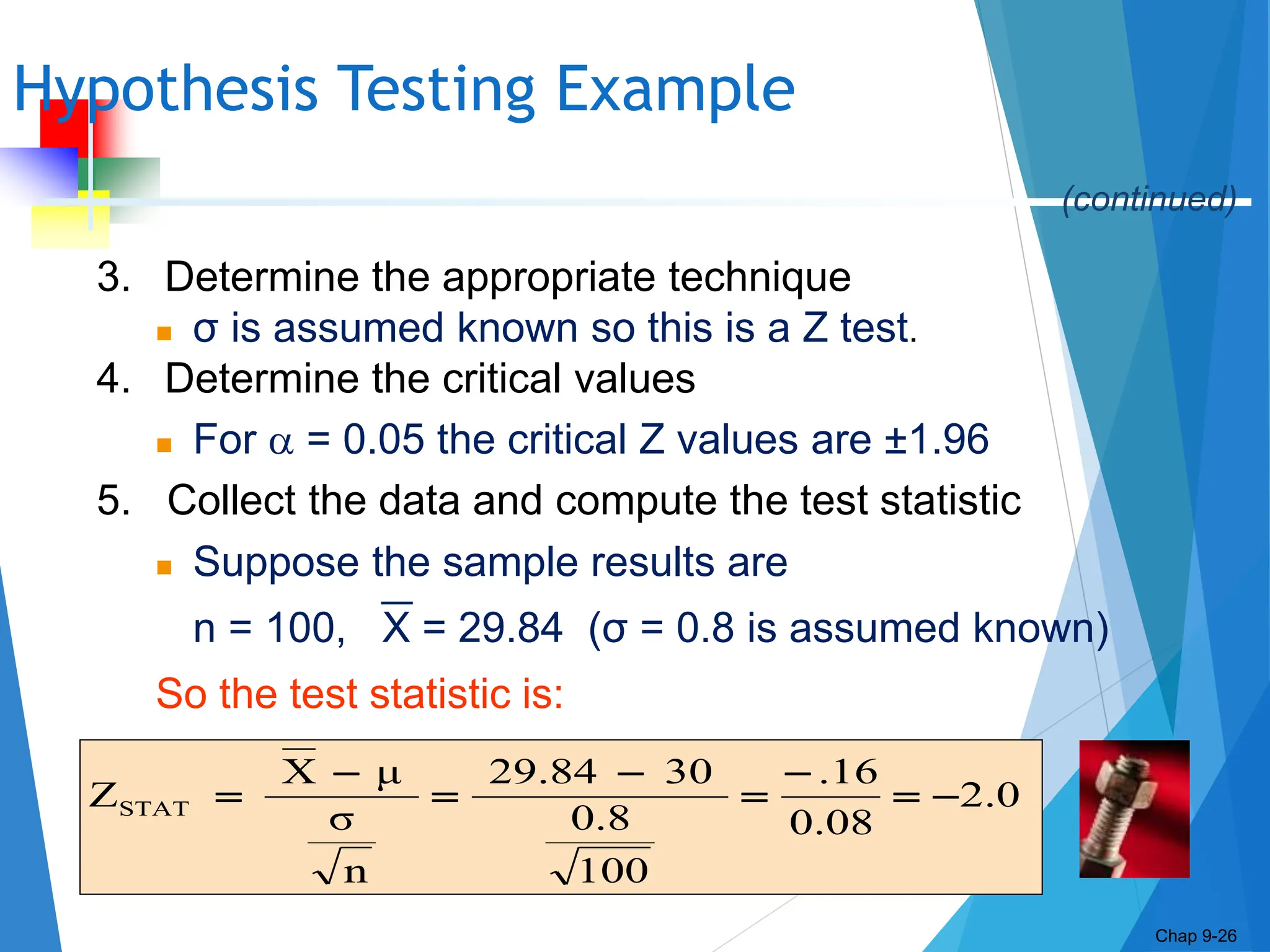
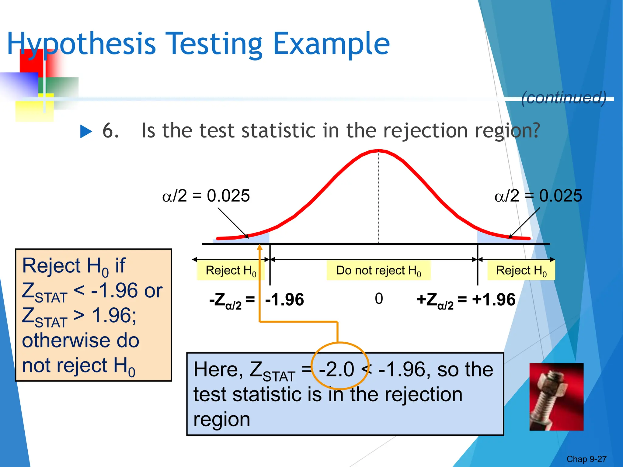
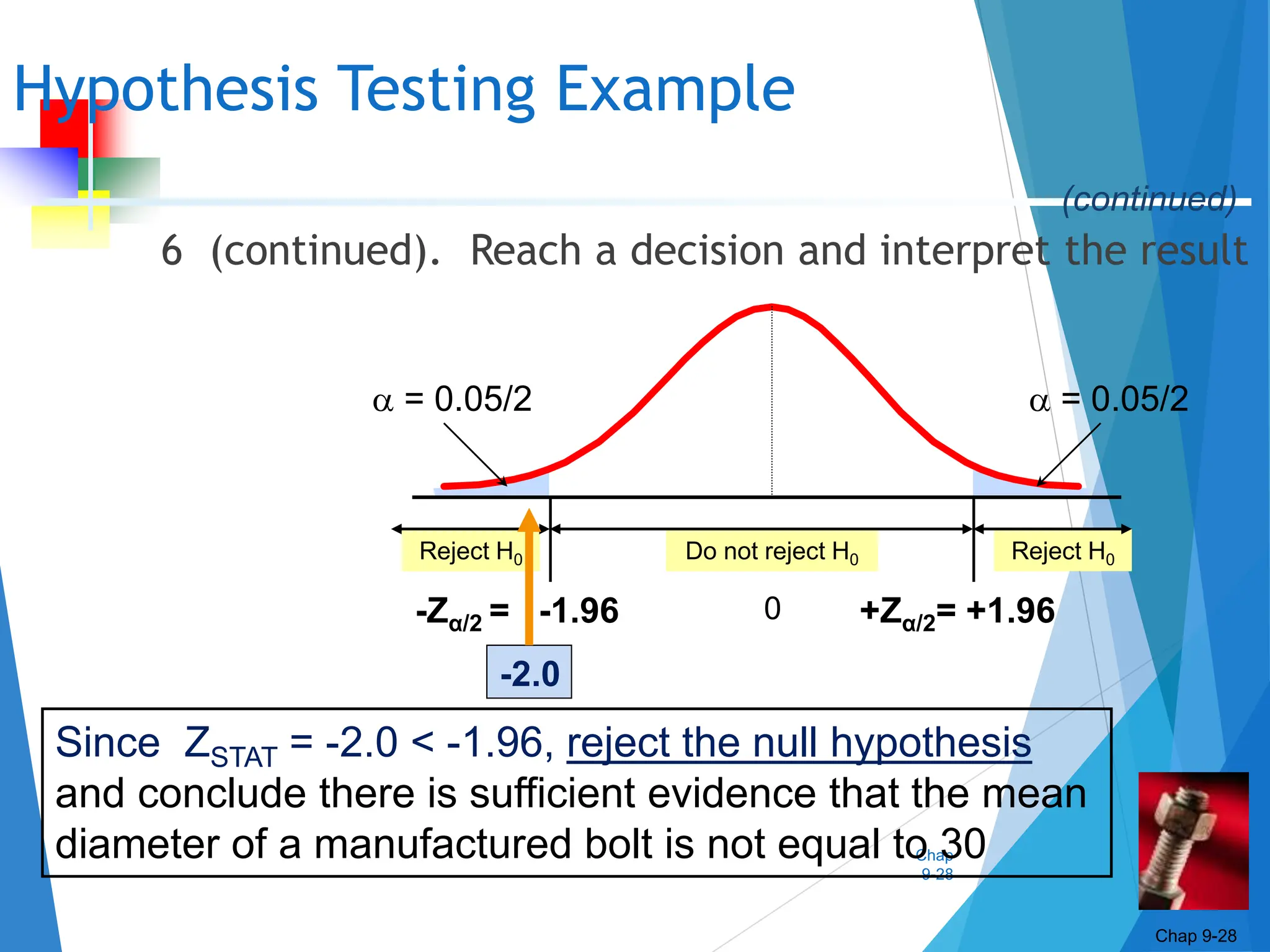
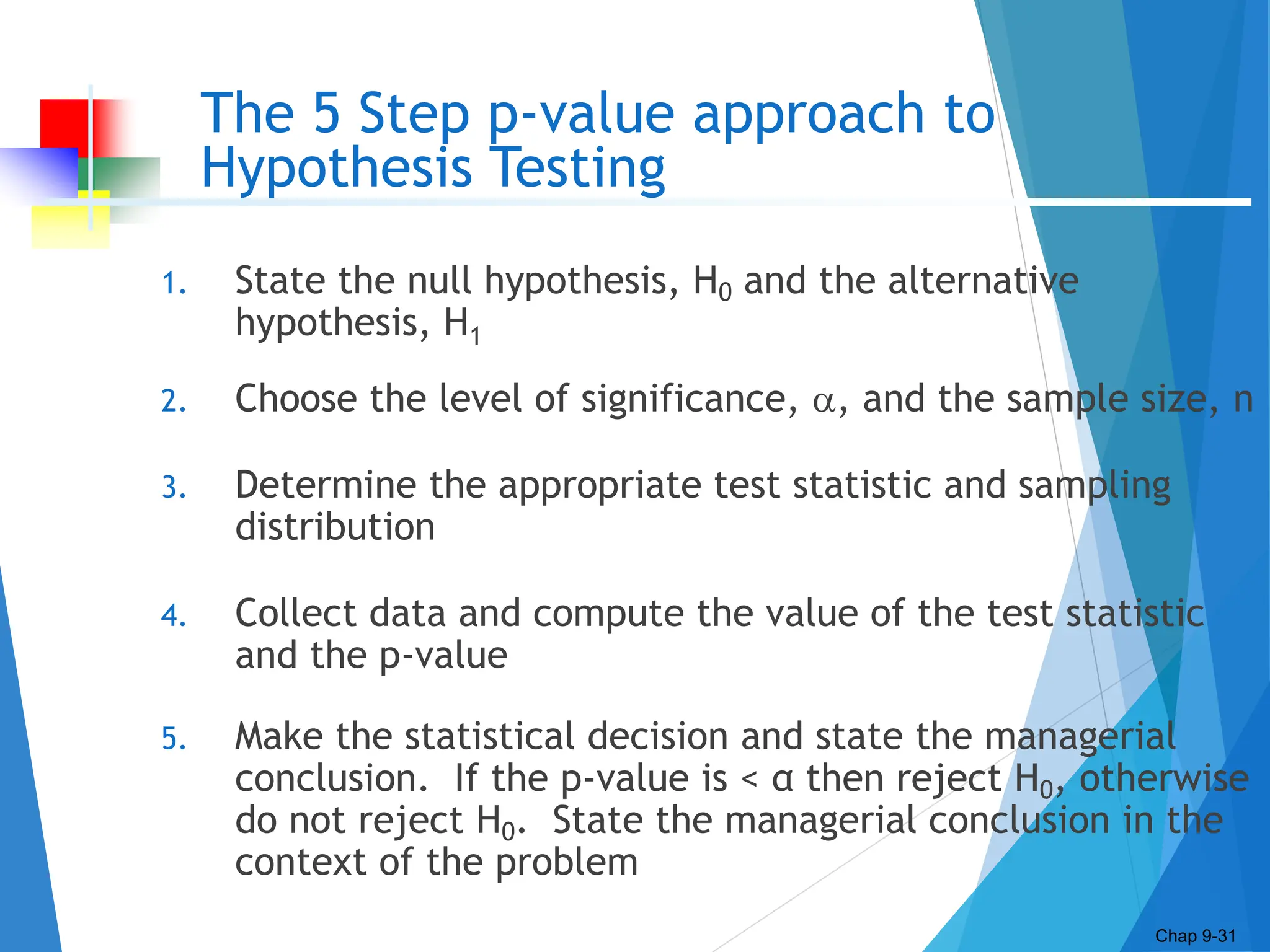
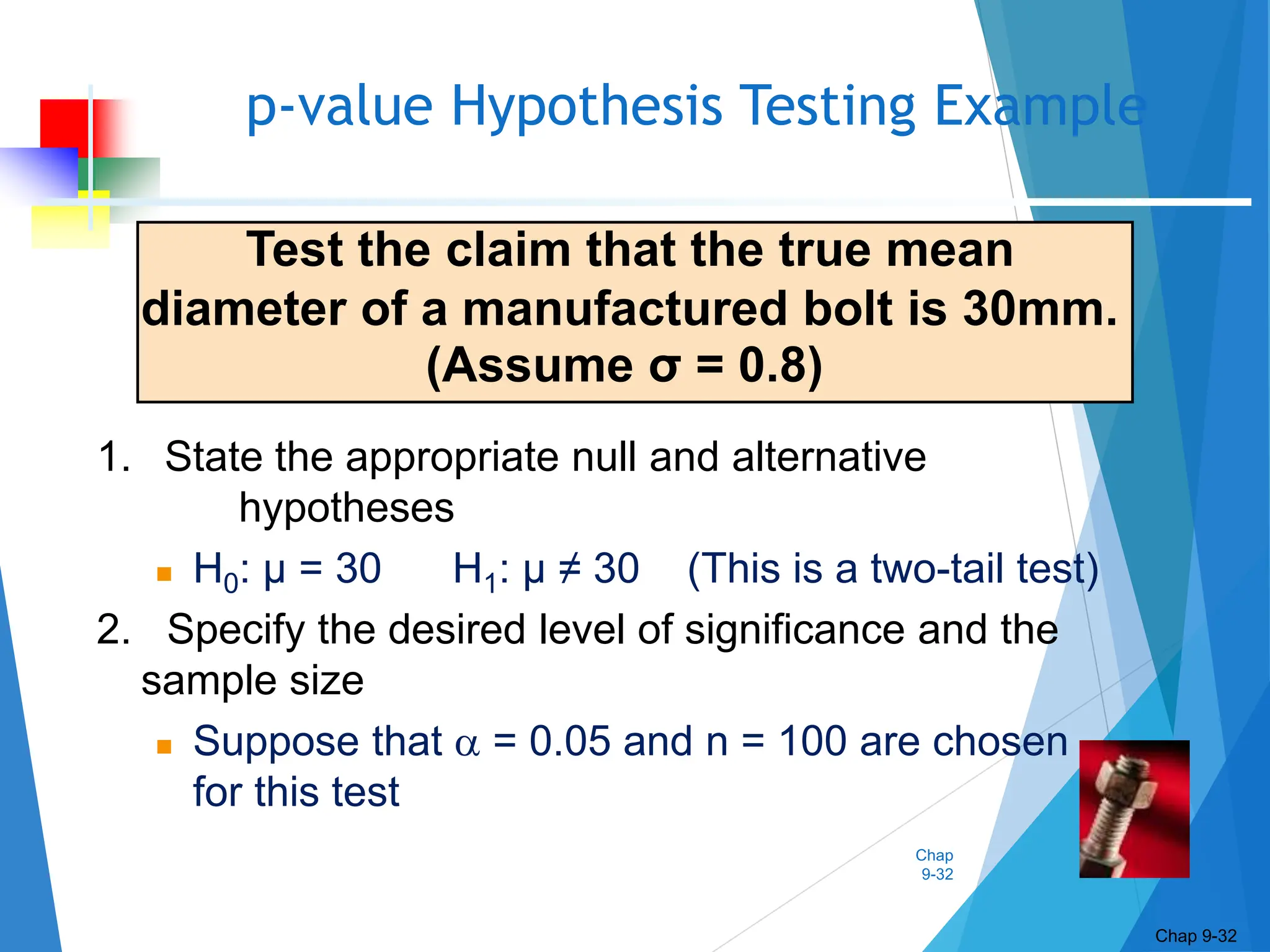
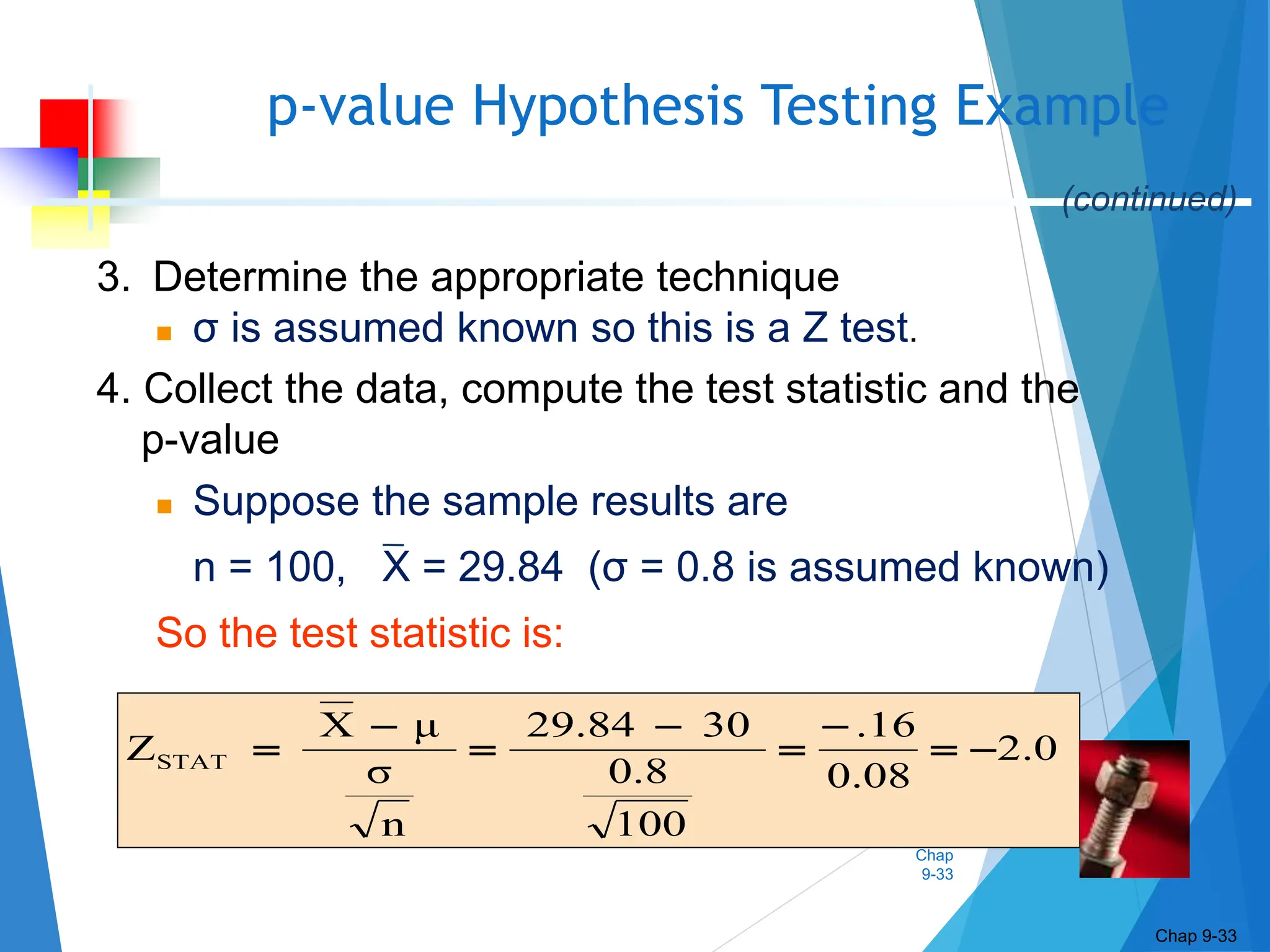
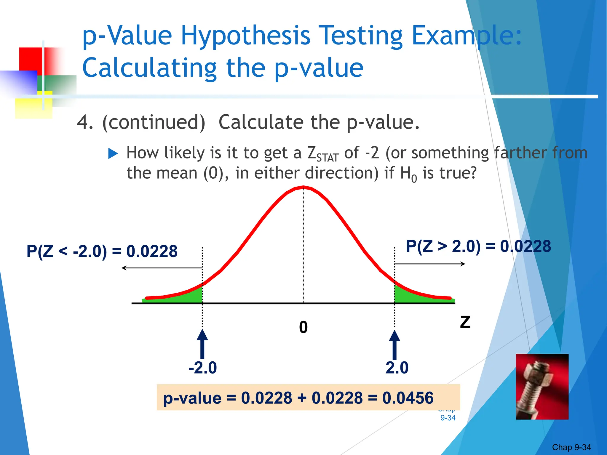
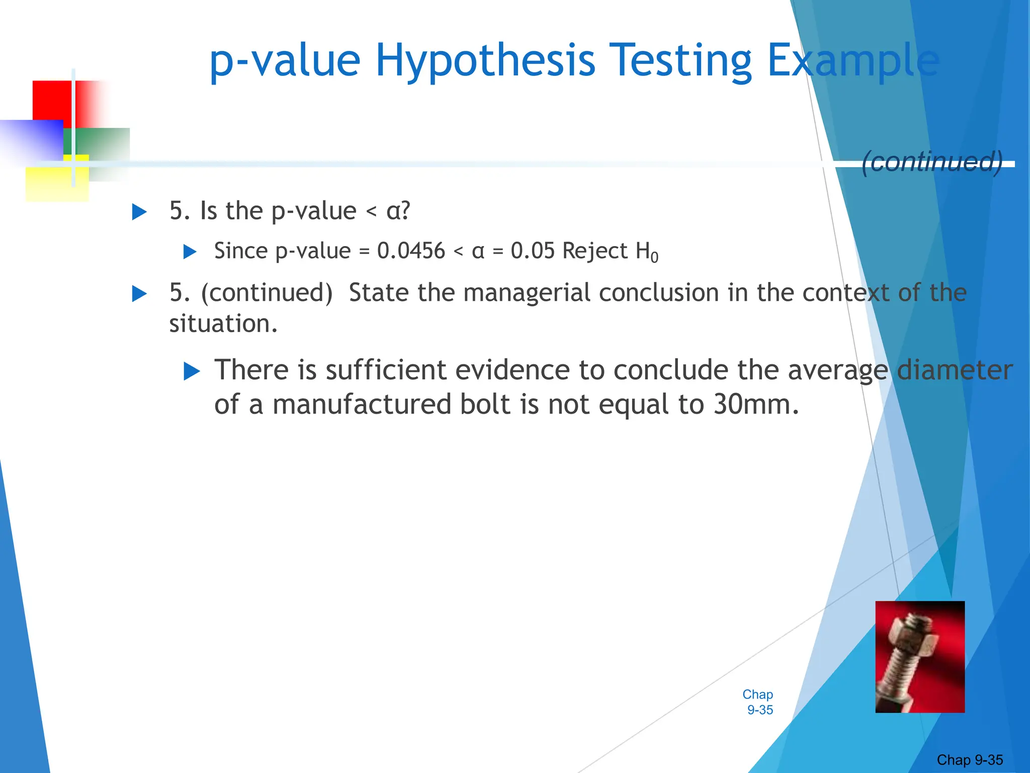
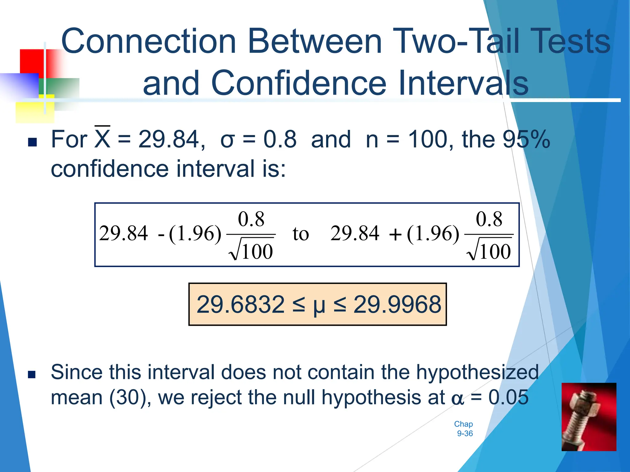
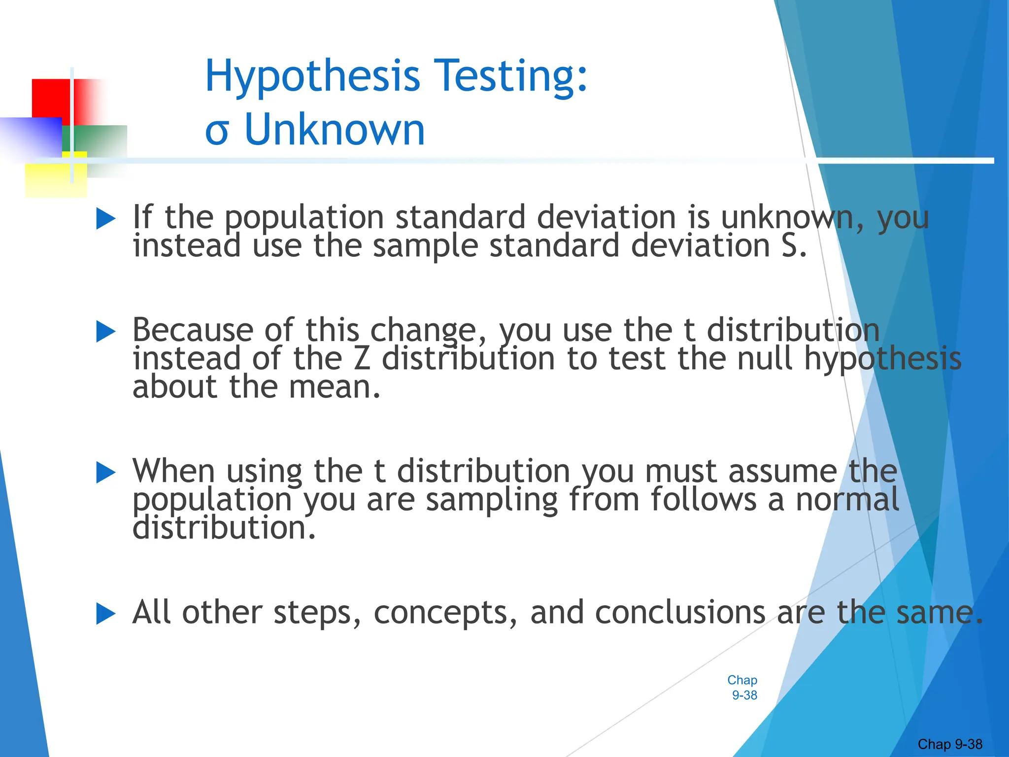
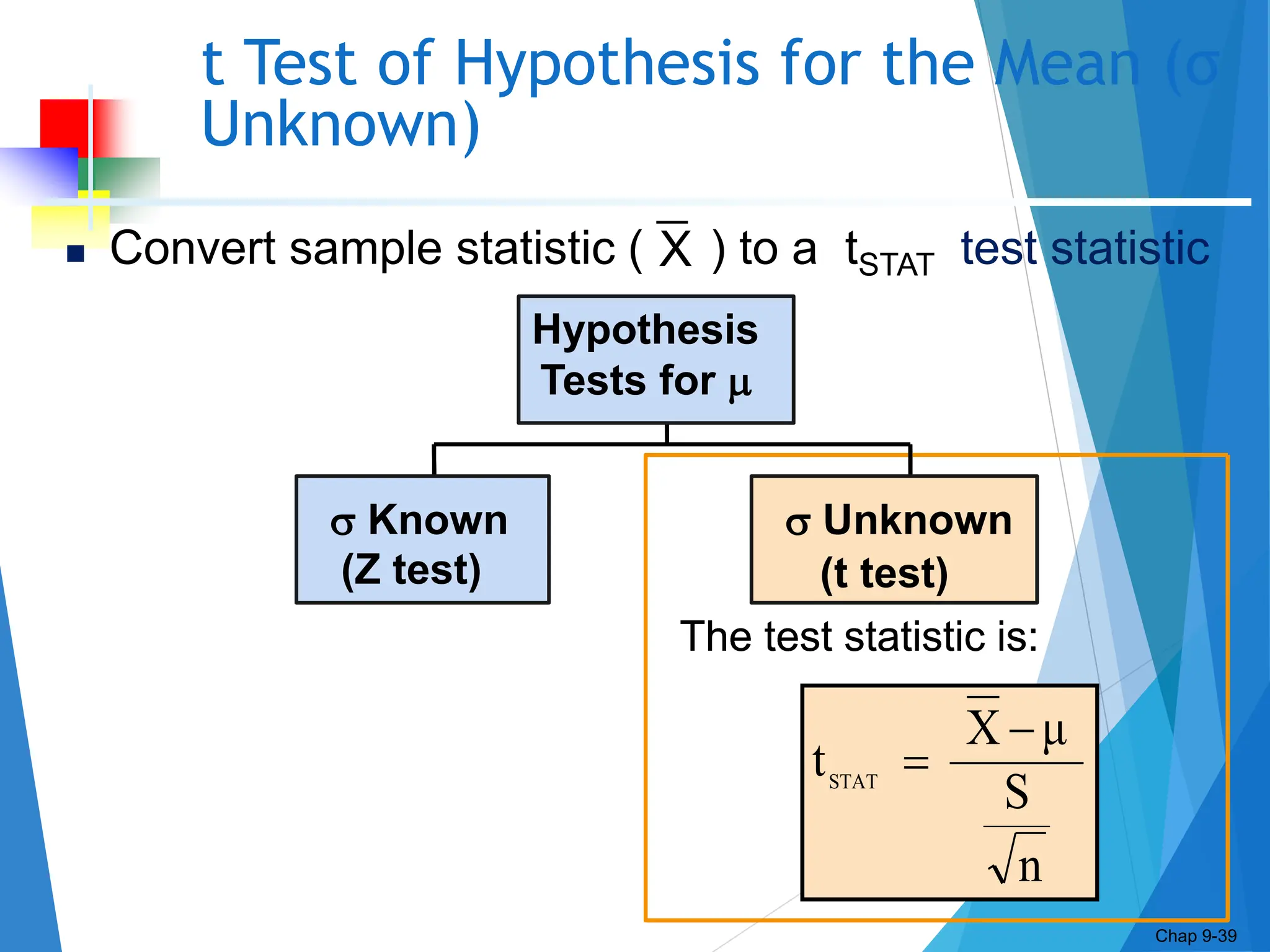
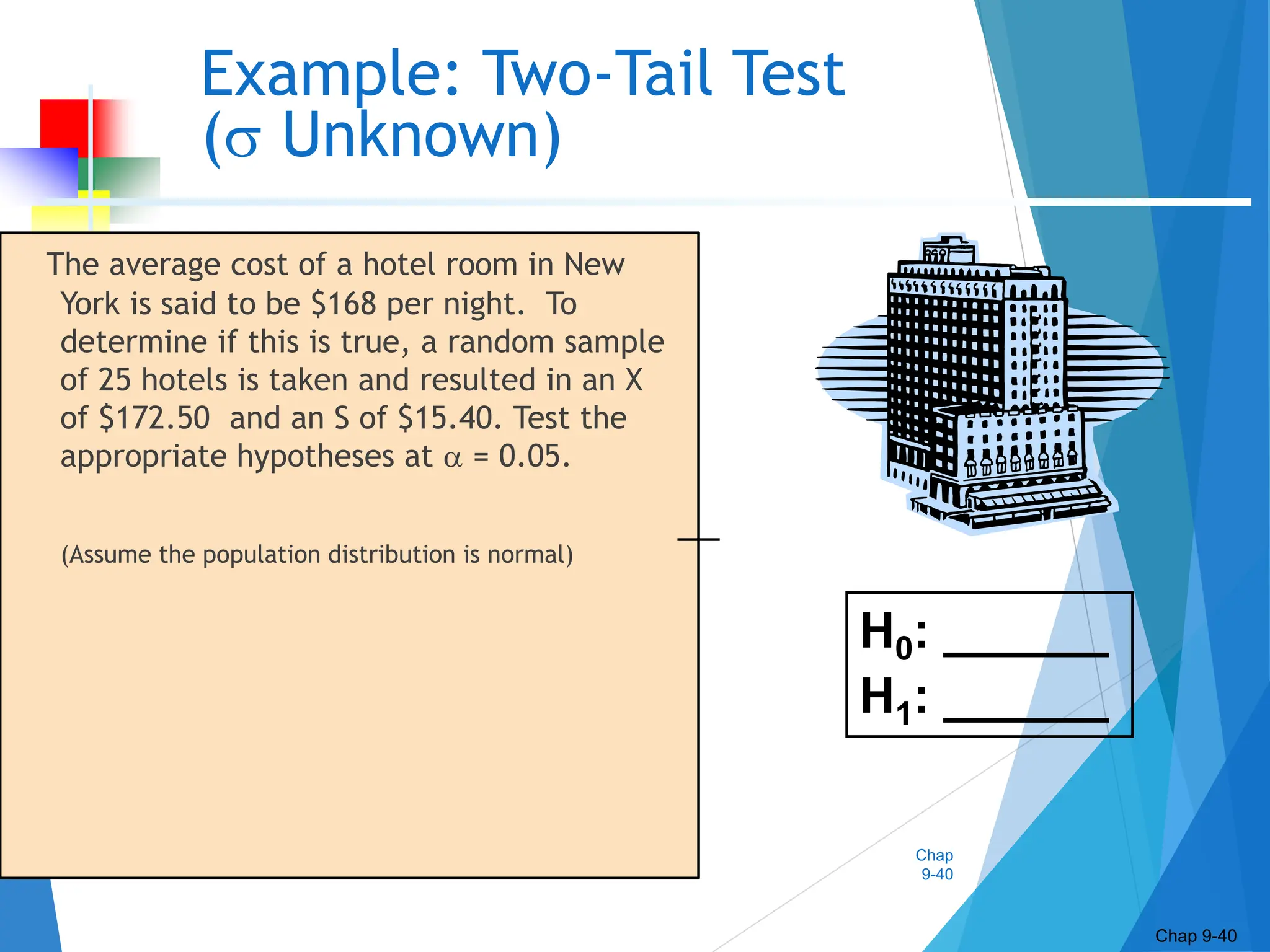
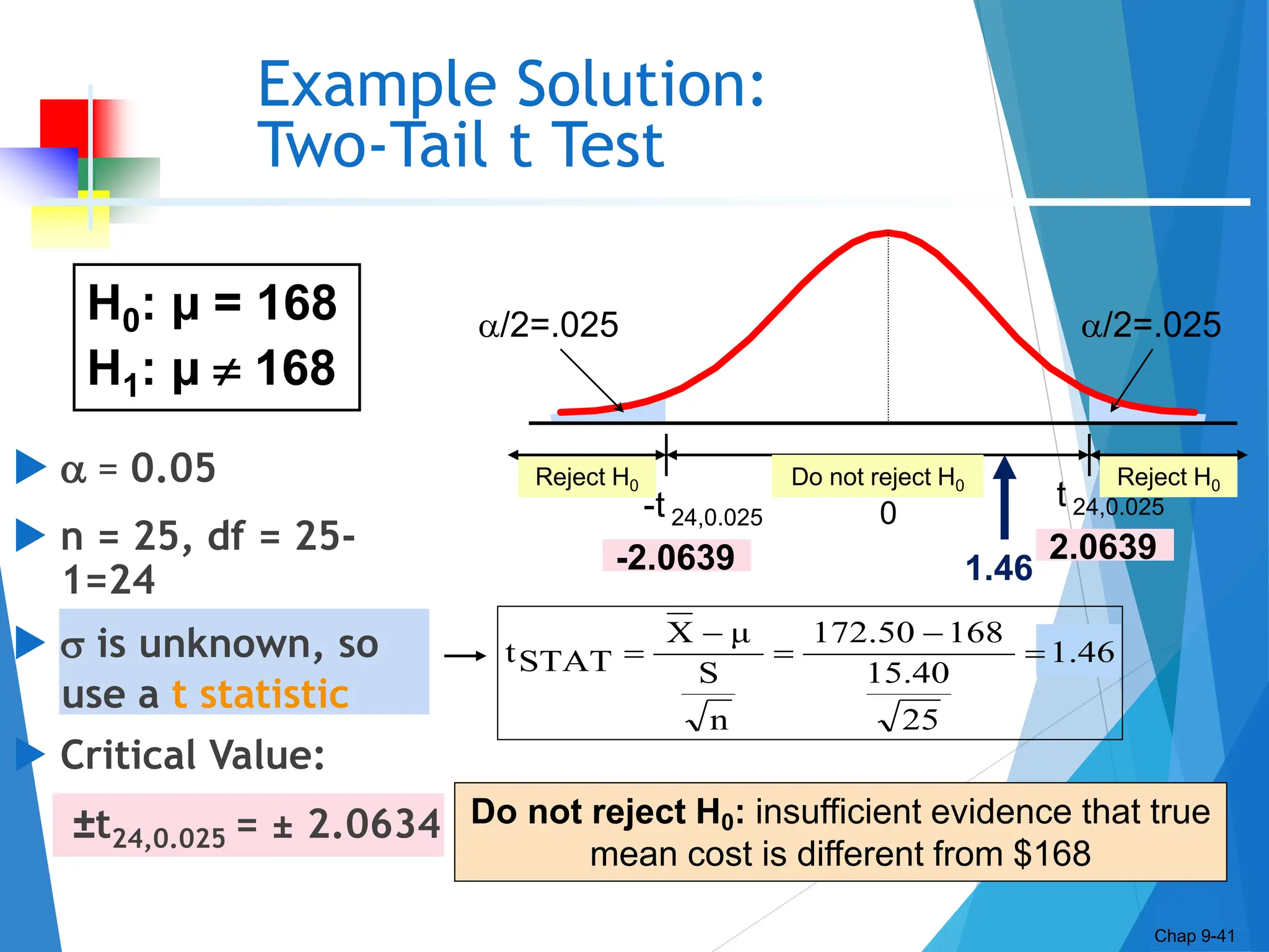
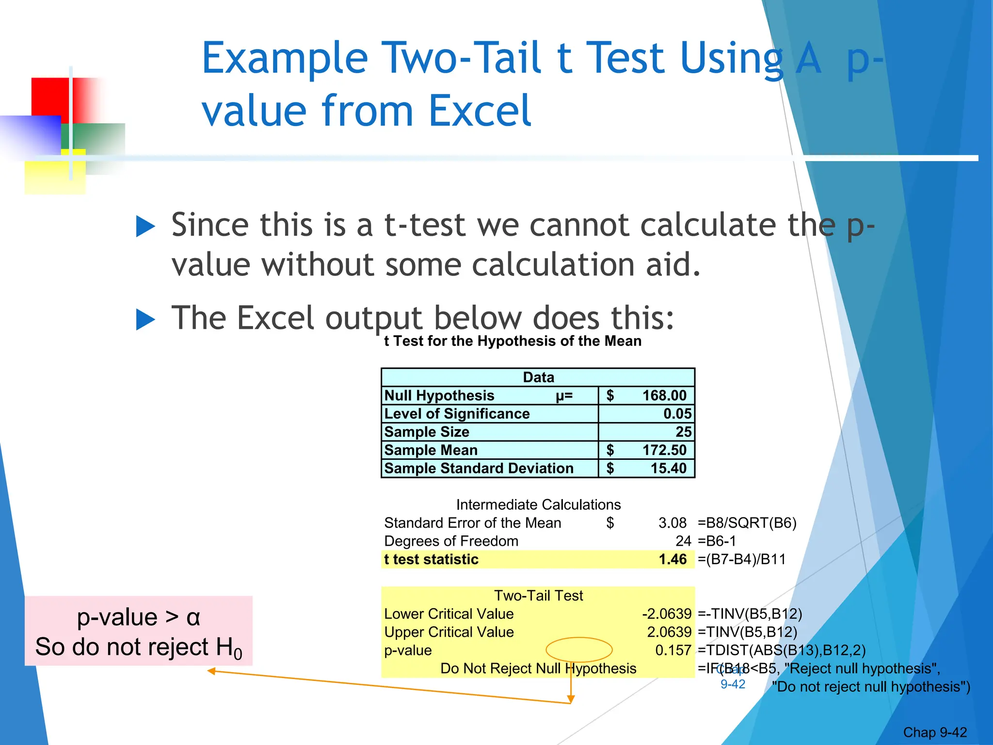
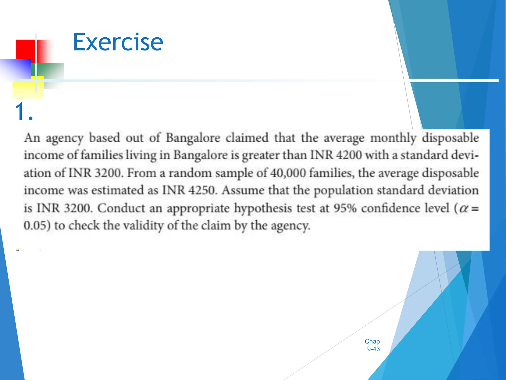
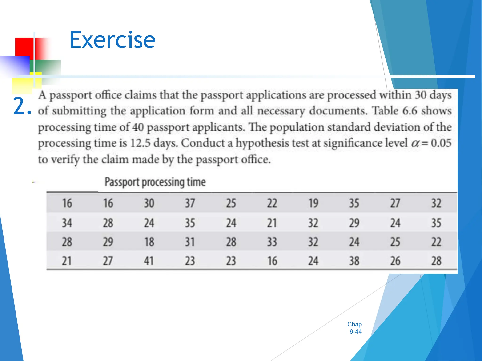
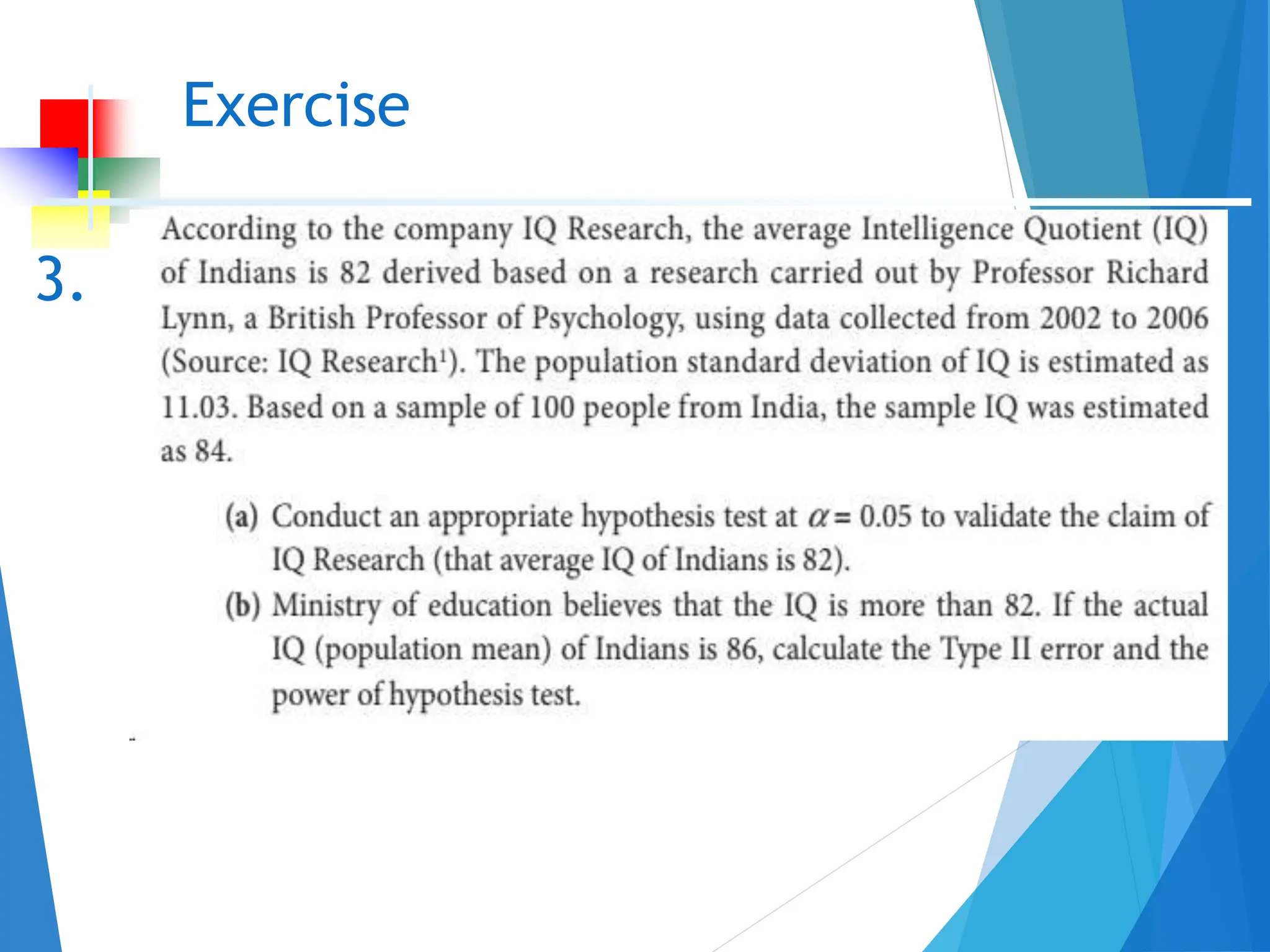
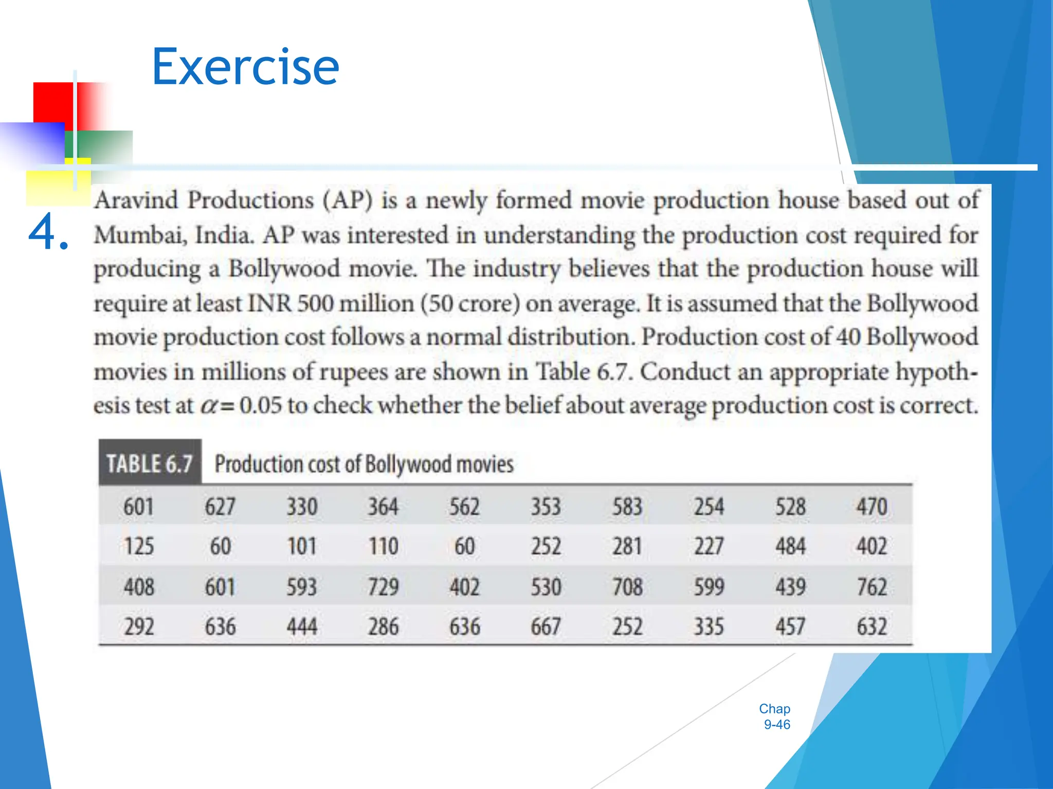
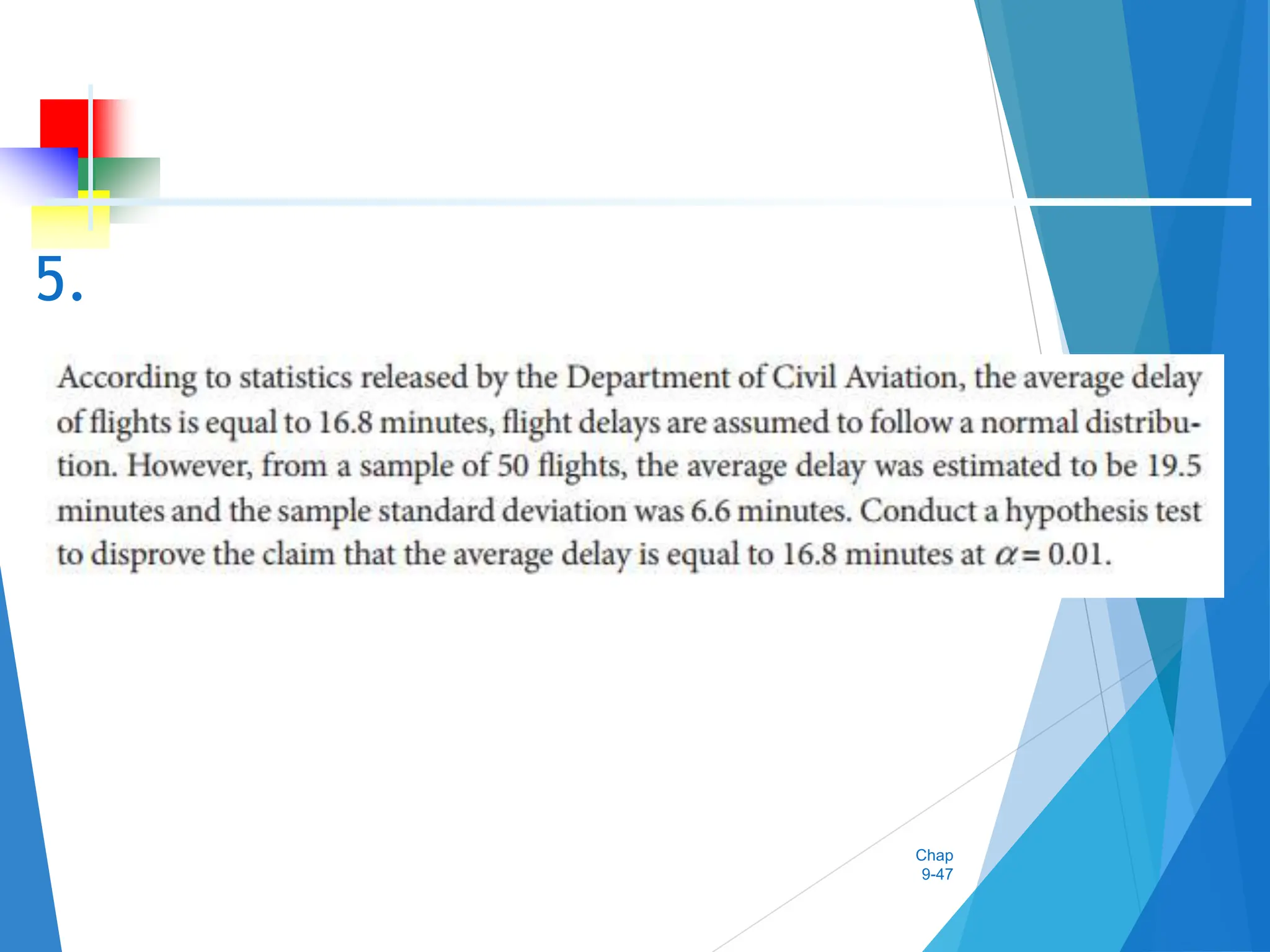
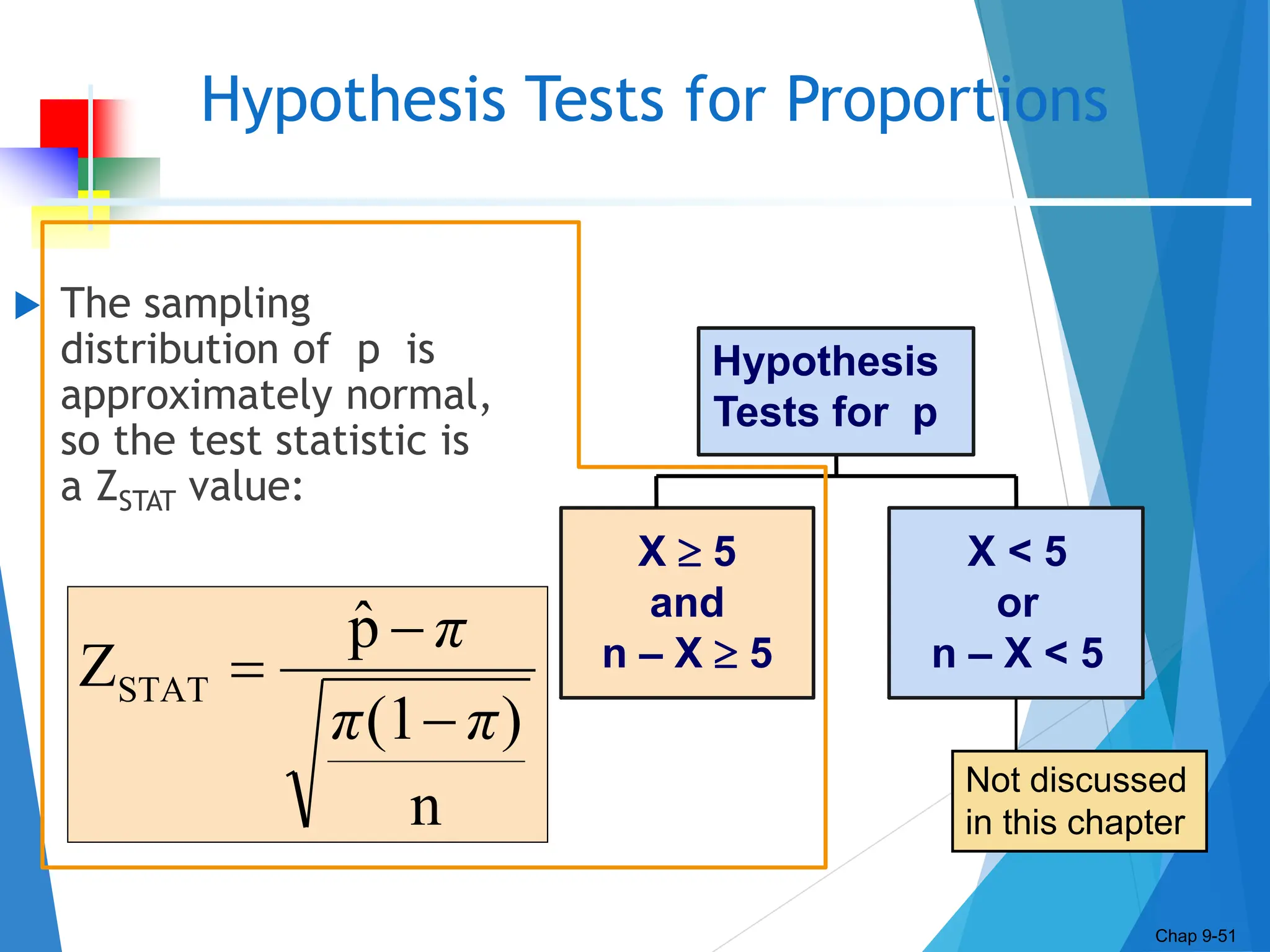
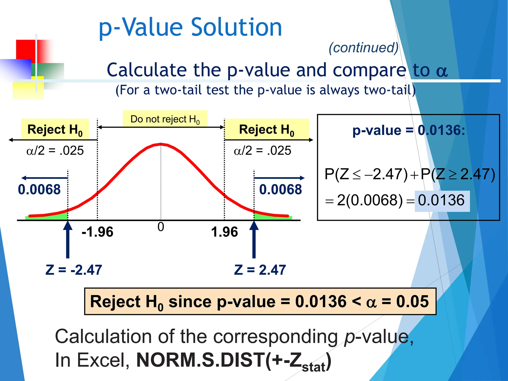
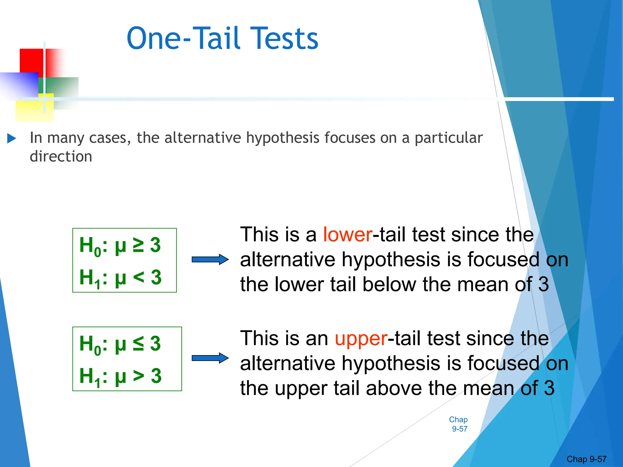
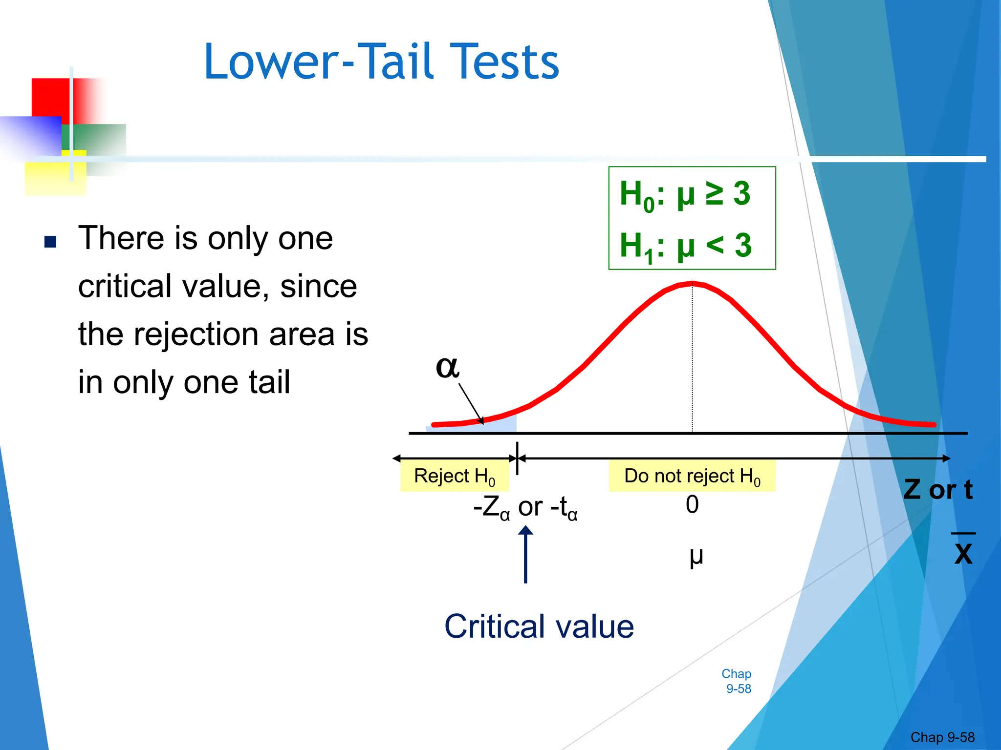
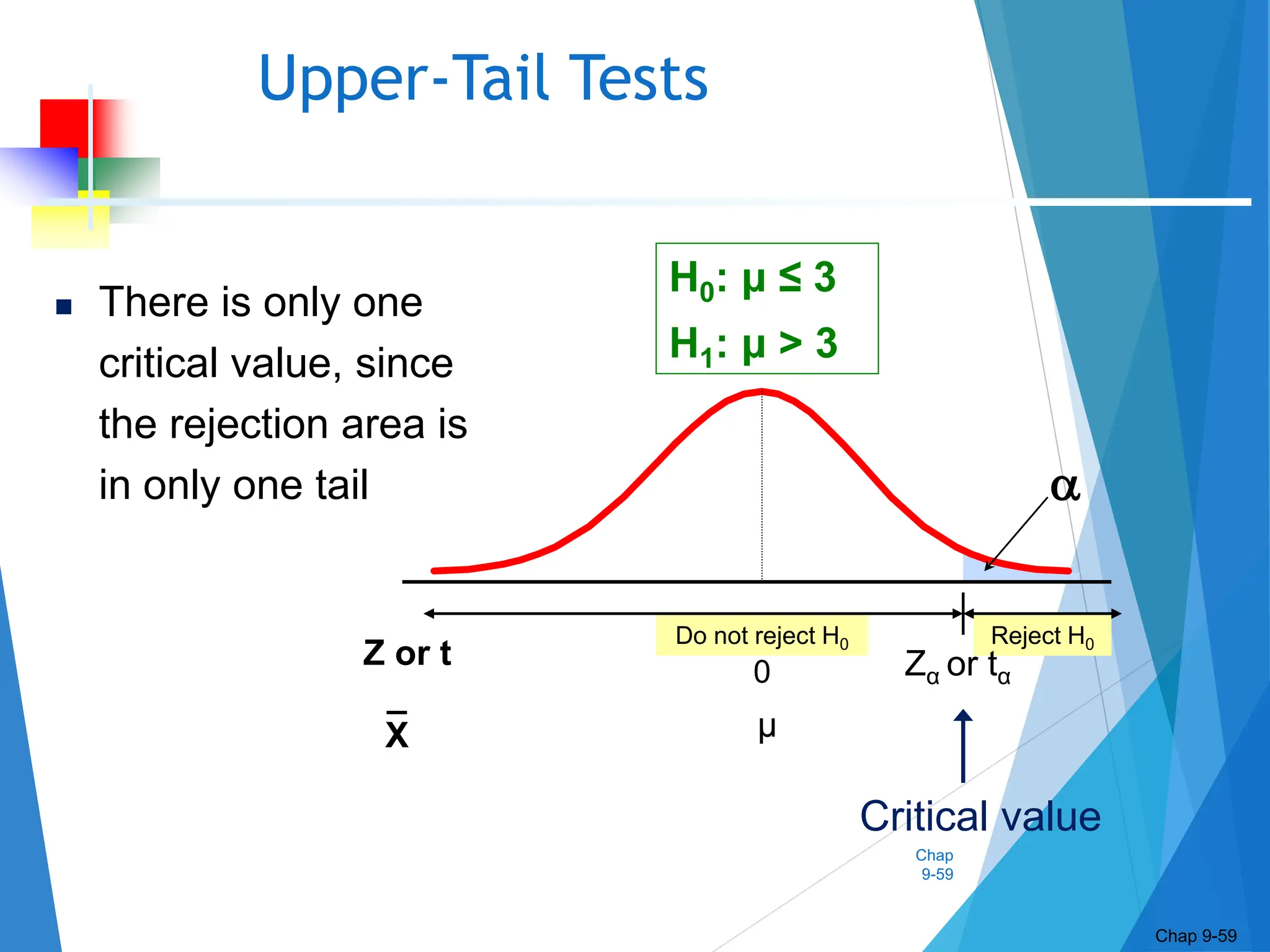
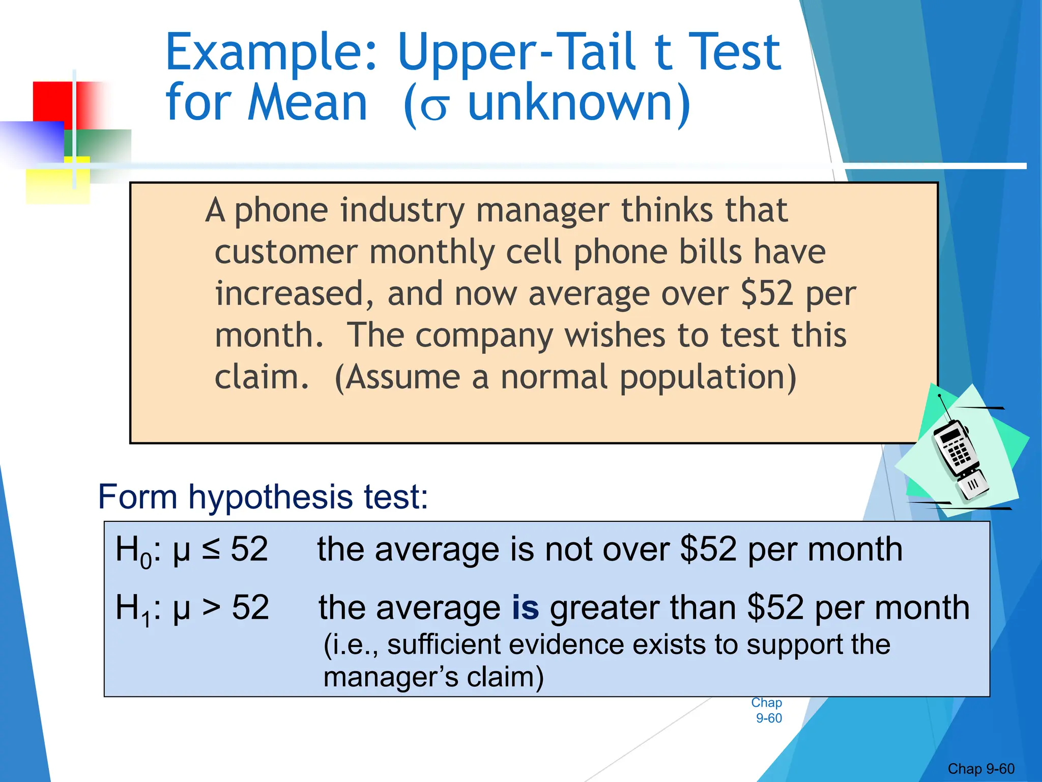
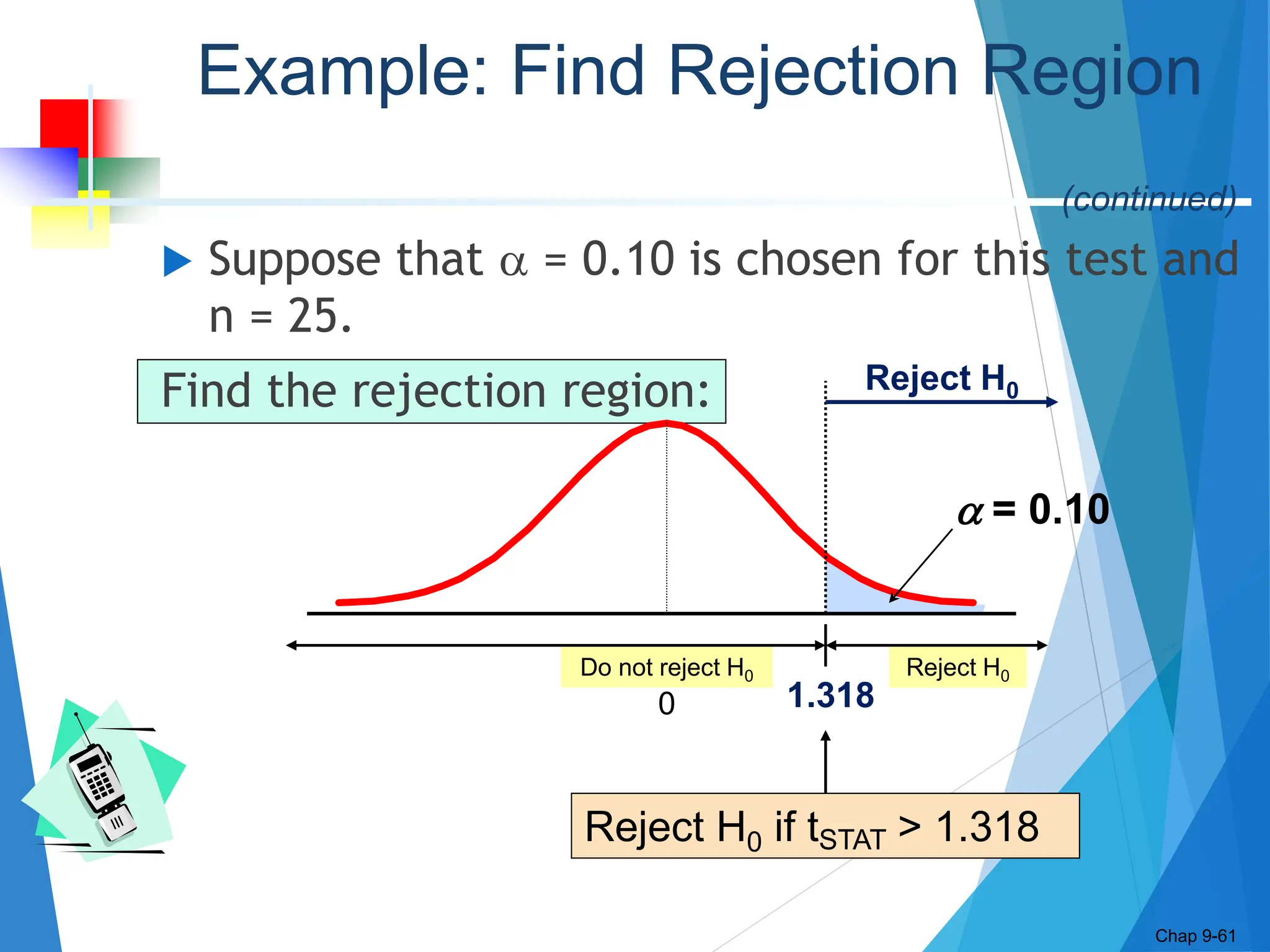
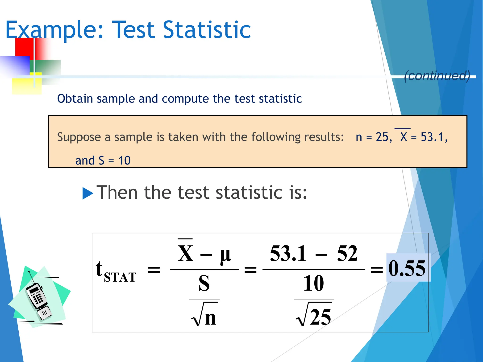
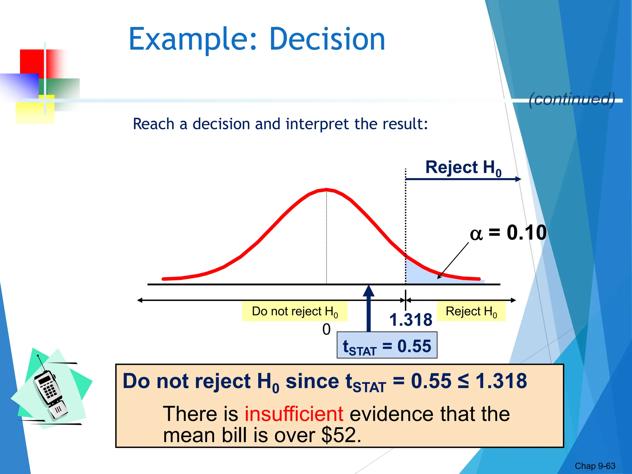
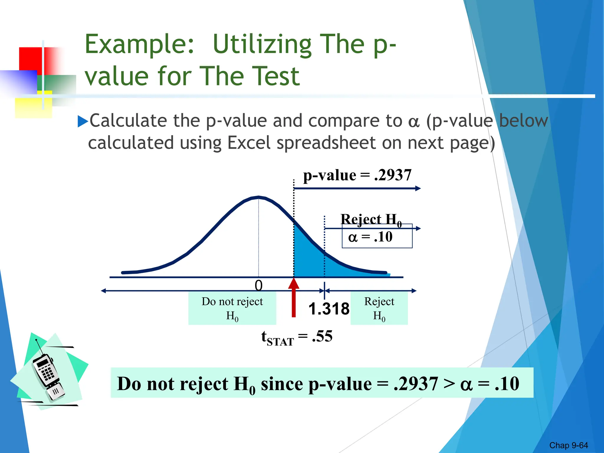
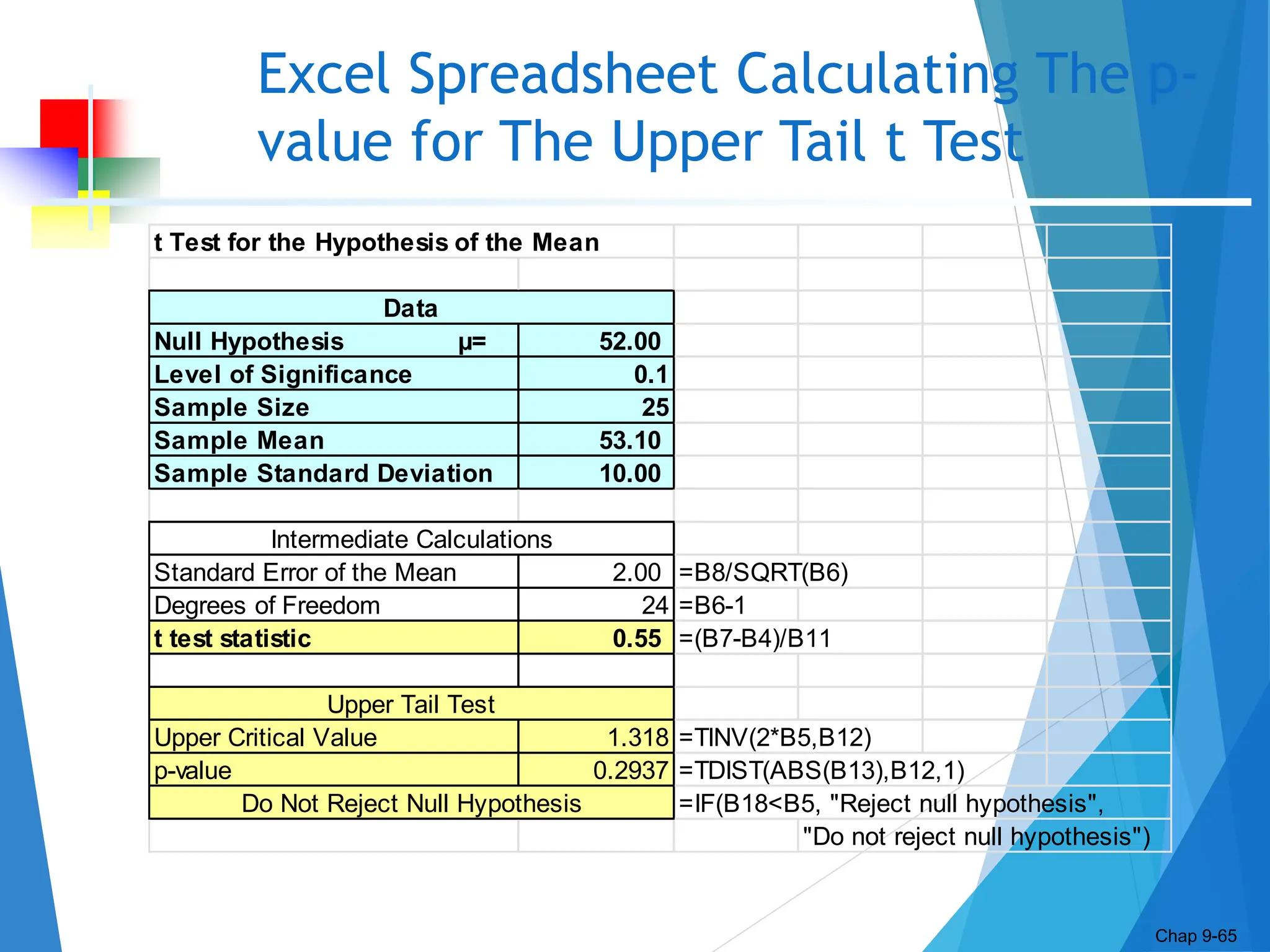
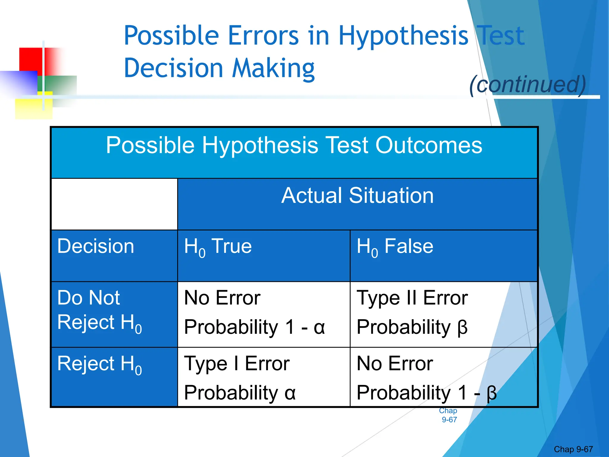
This document discusses hypothesis testing concepts including the null and alternative hypotheses, type I and II errors, and the hypothesis testing process. It provides examples of hypothesis testing for a mean where the population standard deviation is known (z-test) and unknown (t-test). The document outlines the 6 steps in hypothesis testing and provides examples using both the critical value approach and p-value approach. It discusses the relationship between hypothesis testing and confidence intervals.

1. MBMG-7104/ ITHS-2202/ IMAS-3101/
IMHS-3101 @Ravindra Nath Shukla (PhD Scholar) ABV-IIITM

2. Learning Objectives
In this chapter, you learn:
 The basic principles of hypothesis testing
 How to use hypothesis testing to test a mean or
proportion
 The assumptions of each hypothesis-testing
procedure, how to evaluate them, and the
consequences if they are seriously violated
 How to avoid the pitfalls involved in hypothesis
testing
 The ethical issues involved in hypothesis testing
Chap 9-2

3. What is a Hypothesis?
 Hypothesis is a claim made by a
person/organization.
 A hypothesis is a claim (assertion) about a
population parameter such as mean or
proportion and we seek evidence from a
sample for the support of the claim.
 for example, claim could be that the average
salary of analytics experts is at least USD
1,00,000.
 Hypothesis testing is a process used for either
rejecting or retaining a null hypothesis
Chap 9-3

4. Chap
9-4
What is a Hypothesis?
 Suppose :
 population mean
 population proportion
Chap 9-4
Example: The mean monthly cell phone bill
in this city is μ = $42
Example: The proportion of adults in this
city with cell phones is π = 0.68

5. The Null Hypothesis, H0
 States the claim or assertion to be tested
Example: The average diameter of a
manufactured bolt is 30mm ( )
 Is always about a population parameter,
not about a sample statistic
Chap 9-5
30
μ
:
H0 
30
μ
:
H0  30
X
:
H0 

6. The Null Hypothesis, H0
 Begin with the assumption that the null
hypothesis is true
Similar to the notion of innocent until
proven guilty
 Refers to the status quo or historical value
 Null always contains “=“sign
 May or may not be rejected
Chap 9-6
(continued)

7. The Alternative Hypothesis, H1
 Is the opposite of the null hypothesis
 e.g., The average diameter of a manufactured bolt is not equal to
30mm ( H1: μ ≠ 30 )
 Challenges the status quo
 Alternative never contains the “=”sign
 May or may not be proven
 Is generally the hypothesis that the researcher is trying to prove
Chap 9-7

8. Chap
9-8
The Hypothesis Testing Process
 Claim: The population mean age is 50.
 H0: μ = 50, H1: μ ≠ 50
 Sample the population and find sample mean.
Chap 9-8
Population
Sample

9. The Hypothesis Testing Process
 Suppose the sample mean age was X = 20.
 This is significantly lower than the
claimed mean population age of 50.
 If the null hypothesis were true, the
probability of getting such a different
sample mean would be very small, so you
reject the null hypothesis.
 In other words, getting a sample mean of
20 is so unlikely if the population mean
was 50, you conclude that the population
mean must not be 50.
Chap 9-9
(continued)

10. The Hypothesis Testing Process
Chap 9-10
Sampling
Distribution of X
μ = 50
If H0 is true
If it is unlikely that you
would get a sample
mean of this value ...
... then you reject
the null hypothesis
that μ = 50.
20
... When in fact this were
the population mean…
X
(continued)

11. Chap
9-11
The Test Statistic and
Critical Values
 If the sample mean is close to the stated population mean, the null
hypothesis is not rejected.
 If the sample mean is far from the stated population mean, the null
hypothesis is rejected.
 How far is “far enough” to reject H0?
 The critical value of a test statistic creates a “line in the sand” for decision
making -- it answers the question of how far is far enough.
Chap 9-11

12. Chap
9-12
The Test Statistic and
Critical Values
Chap 9-12
Critical Values
“Too Far Away” From Mean of Sampling Distribution
Sampling Distribution of the test statistic
Region of
Rejection
Region of
Rejection
Region of
Non-Rejection

13. Chap
9-13
Possible Errors in Hypothesis Test
Decision Making
 Type I Error
 Reject a true null hypothesis
 Considered a serious type of error
 The probability of a Type I Error is 
Called level of significance of the test
Set by researcher in advance
 Type II Error
 Failure to reject a false null hypothesis
 The probability of a Type II Error is β
Chap 9-13

14. Chap
9-14
Possible Errors in Hypothesis Test
Decision Making
Possible Hypothesis Test Outcomes
Actual Situation
Decision H0 True H0 False
Do Not
Reject H0
No Error
Probability 1 - α
Type II Error
Probability β
Reject H0 Type I Error
Probability α
No Error
Probability 1 - β
Chap 9-14
(continued)

15. Chap
9-15
Possible Errors in Hypothesis Test
Decision Making
 The confidence coefficient (1-α) is the probability of not
rejecting H0 when it is true.
 The confidence level of a hypothesis test is (1-α)*100%.
 The power of a statistical test (1-β) is the probability of
rejecting H0 when it is false.
Chap 9-15
(continued)

16. Chap
9-16
Type I & II Error Relationship
Chap 9-16
 Type I and Type II errors cannot happen at
the same time
 A Type I error can only occur if H0 is true
 A Type II error can only occur if H0 is false
If Type I error probability () , then
Type II error probability (β)

17. Chap
9-17
Factors Affecting Type II Error
 All else equal,
 β when the difference between hypothesized parameter and its
true value
 β when 
 β when σ
 β when n
Chap 9-17

18. Chap
9-18
Level of Significance
and the Rejection Region
Chap 9-18
Level of significance = 
This is a two-tail test because there is a rejection region in both tails
H0: μ = 30
H1: μ ≠ 30
Critical values
Rejection Region
/2
30

/2


19. Chap
9-19
Hypothesis Tests for the Mean
Chap 9-19
 Known  Unknown
Hypothesis
Tests for 
(Z test) (t test)

20. Chap
9-20
Z Test of Hypothesis for the Mean (σ
Known)
 Convert sample statistic ( ) to a ZSTAT test
statistic
Chap 9-20
X
The test statistic is:
n
σ
μ
X
ZSTAT


σ Known σ Unknown
Hypothesis
Tests for 
 Known  Unknown
(Z test) (t test)

21. Chap
9-21
Critical Value
Approach to Testing
 For a two-tail test for the mean, σ known:
 Convert sample statistic ( ) to test statistic (ZSTAT)
 Determine the critical Z values for a specified
level of significance  from a table or computer
 Decision Rule: If the test statistic falls in the rejection region,
reject H0 ; otherwise do not reject H0
Chap 9-21
X

22. Chap
9-22
Two-Tail Tests
Chap 9-22
Do not reject H0 Reject H0
Reject H0
 There are two
cutoff values
(critical values),
defining the
regions of
rejection
/2
-Zα/2 0
H0: μ = 30
H1: μ  30
+Zα/2
/2
Lower
critical
value
Upper
critical
value
30
Z
X

23. 6 Steps in
Hypothesis Testing
1. State the null hypothesis, H0 and the alternative
hypothesis, H1
2. Choose the level of significance, , and the sample size, n
3. Determine the appropriate test statistic and sampling
distribution
4. Determine the critical values that divide the rejection and
non-rejection regions
Chap 9-23

24. 6 Steps in
Hypothesis Testing
5. Collect data and compute the value of the test
statistic
6. Make the statistical decision and state the
managerial conclusion. If the test statistic falls into
the nonrejection region, do not reject the null
hypothesis H0. If the test statistic falls into the
rejection region, reject the null hypothesis. Express
the managerial conclusion in the context of the
problem
Chap 9-24
(continued)

25. Chap
9-25
Hypothesis Testing Example
Chap 9-25
Test the claim that the true mean diameter
of a manufactured bolt is 30mm.
(Assume σ = 0.8)
1. State the appropriate null and alternative
hypotheses
 H0: μ = 30 H1: μ ≠ 30 (This is a two-tail test)
2. Specify the desired level of significance and the
sample size
 Suppose that  = 0.05 and n = 100 are chosen
for this test

26. Chap
9-26
Hypothesis Testing Example
Chap 9-26
2.0
0.08
.16
100
0.8
30
29.84
n
σ
μ
X
ZSTAT 







3. Determine the appropriate technique
 σ is assumed known so this is a Z test.
4. Determine the critical values
 For  = 0.05 the critical Z values are ±1.96
5. Collect the data and compute the test statistic
 Suppose the sample results are
n = 100, X = 29.84 (σ = 0.8 is assumed known)
So the test statistic is:
(continued)

27. Chap
9-27
 6. Is the test statistic in the rejection region?
Hypothesis Testing Example
Chap 9-27
Reject H0 Do not reject H0
/2 = 0.025
-Zα/2 = -1.96 0
Reject H0 if
ZSTAT < -1.96 or
ZSTAT > 1.96;
otherwise do
not reject H0
(continued)
/2 = 0.025
Reject H0
+Zα/2 = +1.96
Here, ZSTAT = -2.0 < -1.96, so the
test statistic is in the rejection
region

28. Chap
9-28
6 (continued). Reach a decision and interpret the result
Hypothesis Testing Example
Chap 9-28
-2.0
Since ZSTAT = -2.0 < -1.96, reject the null hypothesis
and conclude there is sufficient evidence that the mean
diameter of a manufactured bolt is not equal to 30
(continued)
Reject H0 Do not reject H0
 = 0.05/2
-Zα/2 = -1.96 0
 = 0.05/2
Reject H0
+Zα/2= +1.96

29. Chap
9-29
p-Value Approach to Testing
 p-value: Probability of obtaining a test statistic equal to or more
extreme than the observed sample value given H0 is true
 The p-value is also called the observed level of significance
 H0 can be rejected if the p-value is less than α
Chap 9-29

30. Chap
9-30
p-Value Approach to Testing:
Interpreting the p-value
 Compare the p-value with 
 If p-value <  , reject H0
 If p-value   , do not reject H0
 Remember
If the p-value is low then H0 must go
Chap 9-30

31. The 5 Step p-value approach to
Hypothesis Testing
1. State the null hypothesis, H0 and the alternative
hypothesis, H1
2. Choose the level of significance, , and the sample size, n
3. Determine the appropriate test statistic and sampling
distribution
4. Collect data and compute the value of the test statistic
and the p-value
5. Make the statistical decision and state the managerial
conclusion. If the p-value is < α then reject H0, otherwise
do not reject H0. State the managerial conclusion in the
context of the problem
Chap 9-31

32. Chap
9-32
p-value Hypothesis Testing Example
Chap 9-32
Test the claim that the true mean
diameter of a manufactured bolt is 30mm.
(Assume σ = 0.8)
1. State the appropriate null and alternative
hypotheses
 H0: μ = 30 H1: μ ≠ 30 (This is a two-tail test)
2. Specify the desired level of significance and the
sample size
 Suppose that  = 0.05 and n = 100 are chosen
for this test

33. Chap
9-33
p-value Hypothesis Testing Example
Chap 9-33
2.0
0.08
.16
100
0.8
30
29.84
n
σ
μ
X
ZSTAT 







3. Determine the appropriate technique
 σ is assumed known so this is a Z test.
4. Collect the data, compute the test statistic and the
p-value
 Suppose the sample results are
n = 100, X = 29.84 (σ = 0.8 is assumed known)
So the test statistic is:
(continued)

34. Chap
9-34
p-Value Hypothesis Testing Example:
Calculating the p-value
4. (continued) Calculate the p-value.
 How likely is it to get a ZSTAT of -2 (or something farther from
the mean (0), in either direction) if H0 is true?
Chap 9-34
p-value = 0.0228 + 0.0228 = 0.0456
P(Z < -2.0) = 0.0228
0
-2.0
Z
2.0
P(Z > 2.0) = 0.0228

35. Chap
9-35
 5. Is the p-value < α?
 Since p-value = 0.0456 < α = 0.05 Reject H0
 5. (continued) State the managerial conclusion in the context of the
situation.
 There is sufficient evidence to conclude the average diameter
of a manufactured bolt is not equal to 30mm.
p-value Hypothesis Testing Example
Chap 9-35
(continued)

36. Chap
9-36
Connection Between Two-Tail Tests
and Confidence Intervals
 For X = 29.84, σ = 0.8 and n = 100, the 95%
confidence interval is:
29.6832 ≤ μ ≤ 29.9968
 Since this interval does not contain the hypothesized
mean (30), we reject the null hypothesis at  = 0.05
100
0.8
(1.96)
29.84
to
100
0.8
(1.96)
-
29.84 

37. Chap
9-37
Do You Ever Truly Know σ?
 Probably not!
 In virtually all real world business situations, σ is not
known.
 If there is a situation where σ is known then µ is also
known (since to calculate σ you need to know µ.)
 If you truly know µ there would be no need to gather a
sample to estimate it.
Chap 9-37

38. Chap
9-38
Hypothesis Testing:
σ Unknown
 If the population standard deviation is unknown, you
instead use the sample standard deviation S.
 Because of this change, you use the t distribution
instead of the Z distribution to test the null hypothesis
about the mean.
 When using the t distribution you must assume the
population you are sampling from follows a normal
distribution.
 All other steps, concepts, and conclusions are the same.
Chap 9-38

39. Chap
9-39
t Test of Hypothesis for the Mean (σ
Unknown)
Chap 9-39
The test statistic is:
Hypothesis
Tests for 
σ Known σ Unknown
 Known  Unknown
(Z test) (t test)
 Convert sample statistic ( ) to a tSTAT test statistic
The test statistic is:
Hypothesis
Tests for 
σ Known σ Unknown
 Known  Unknown
(Z test) (t test)
X
The test statistic is:
n
S
μ
X
tSTAT


Hypothesis
Tests for 
σ Known σ Unknown
 Known  Unknown
(Z test) (t test)

40. Chap
9-40
Example: Two-Tail Test
( Unknown)
The average cost of a hotel room in New
York is said to be $168 per night. To
determine if this is true, a random sample
of 25 hotels is taken and resulted in an X
of $172.50 and an S of $15.40. Test the
appropriate hypotheses at  = 0.05.
(Assume the population distribution is normal)
Chap 9-40
H0: ______
H1: ______

41. Chap
9-41
  = 0.05
 n = 25, df = 25-
1=24
  is unknown, so
use a t statistic
 Critical Value:
±t24,0.025 = ± 2.0634
Example Solution:
Two-Tail t Test
Chap 9-41
Do not reject H0: insufficient evidence that true
mean cost is different from $168
Reject H0
Reject H0
/2=.025
-t 24,0.025
Do not reject H0
0
/2=.025
-2.0639 2.0639
1.46
25
15.40
168
172.50
n
S
μ
X
STAT
t 




1.46
H0: μ = 168
H1: μ  168
t 24,0.025

42. Chap
9-42
Example Two-Tail t Test Using A p-
value from Excel
 Since this is a t-test we cannot calculate the p-
value without some calculation aid.
 The Excel output below does this:
t Test for the Hypothesis of the Mean
Null Hypothesis µ= 168.00
$
Level of Significance 0.05
Sample Size 25
Sample Mean 172.50
$
Sample Standard Deviation 15.40
$
Standard Error of the Mean 3.08
$ =B8/SQRT(B6)
Degrees of Freedom 24 =B6-1
t test statistic 1.46 =(B7-B4)/B11
Lower Critical Value -2.0639 =-TINV(B5,B12)
Upper Critical Value 2.0639 =TINV(B5,B12)
p-value 0.157 =TDIST(ABS(B13),B12,2)
=IF(B18<B5, "Reject null hypothesis",
"Do not reject null hypothesis")
Data
Intermediate Calculations
Two-Tail Test
Do Not Reject Null Hypothesis
Chap 9-42
p-value > α
So do not reject H0

43. Chap
9-43
Exercise
1.

44. Chap
9-44
Exercise
2.

45. Exercise
3.

46. Chap
9-46
Exercise
4.

47. Chap
9-47
5.

48. Hypothesis Tests for Proportions
 Involves categorical variables
 Two possible outcomes
 Possesses characteristic of interest (probability p)
 Does not possess characteristic of interest (1-p)
 The hypothesis testing for population
proportion based on one sample is also
known as one-sample test for proportion
 Fraction or proportion of the population in
the category of interest is denoted by π
Chap 9-48

49. Hypothesis Tests for Proportions
 According to the central limit theorem of
proportions, the sampling distribution of
proportions 𝑝 for a large sample follows an
approximate normal distribution with mean
π (the population proportion) and standard
deviation
π (1−π)
𝑛
.
 Thus , the Z-statistic is defined as :
𝑍 =
𝑝 − π
π (1 − π)
𝑛
 It will follow a standard normal distribution.
Chap 9-49

50. Proportions
 Sample proportion in the category of interest is
denoted by p

 When both X and n – X are at least 5, p can be
approximated by a normal distribution with mean
and standard deviation

Chap 9-50
size
sample
sample
in
interest
of
category
in
number
n
X
p̂ 



p
μ
n
)
(1
σ

 

p

51.  The sampling
distribution of p is
approximately normal,
so the test statistic is
a ZSTAT value:
Hypothesis Tests for Proportions
Chap 9-51
n
)
(1
p̂
ZSTAT
π
π
π



X  5
and
n – X  5
Hypothesis
Tests for p
X < 5
or
n – X < 5
Not discussed
in this chapter

52.  An equivalent form
to the last slide,
but in terms of the
number in the
category of
interest, X:
Z Test for Proportion in Terms of
Number in Category of Interest
Chap 9-52
)
(1
n
n
X
ZSTAT






X  5
and
n-X  5
Hypothesis
Tests for X
X < 5
or
n-X < 5
Not discussed
in this chapter

53. Example: Z Test for Proportion
A marketing company
claims that it receives
responses from 8% of
those surveyed. To test
this claim, a random
sample of 500 were
surveyed with 25
responses. Test at the 
= 0.05 significance
level.
Chap 9-53
Check:
X = 25
n-X = 475


54. Chap
9-54
Z Test for Proportion: Solution
 = 0.05
n = 500, p = 0.05
Chap 9-54
Reject H0 at  = 0.05
H0: π = 0.08
H1: π  0.08
Critical Values: ± 1.96
Test Statistic:
Decision:
Conclusion:
z
0
Reject Reject
.025
.025
1.96
-2.47
There is sufficient
evidence to reject the
company’s claim of 8%
response rate.
2.47
500
.08)
.08(1
.08
.05
n
)
(1
p̂
ZSTAT 










-1.96

55. Calculate the p-value and compare to 
(For a two-tail test the p-value is always two-tail)
p-Value Solution
Do not reject H0
Reject H0
Reject H0
/2 = .025
1.96
0
Z = -2.47
(continued)
0.0136
2(0.0068)
2.47)
P(Z
2.47)
P(Z






p-value = 0.0136:
Reject H0 since p-value = 0.0136 <  = 0.05
Z = 2.47
-1.96
/2 = .025
0.0068
0.0068
Calculation of the corresponding p-value,
In Excel, NORM.S.DIST(+-Zstat)

56. Chap
9-56

57. Chap
9-57
One-Tail Tests
 In many cases, the alternative hypothesis focuses on a particular
direction
Chap 9-57
H0: μ ≥ 3
H1: μ < 3
H0: μ ≤ 3
H1: μ > 3
This is a lower-tail test since the
alternative hypothesis is focused on
the lower tail below the mean of 3
This is an upper-tail test since the
alternative hypothesis is focused on
the upper tail above the mean of 3

58. Chap
9-58
Lower-Tail Tests
Chap 9-58
Reject H0 Do not reject H0
 There is only one
critical value, since
the rejection area is
in only one tail 
-Zα or -tα 0
μ
H0: μ ≥ 3
H1: μ < 3
Z or t
X
Critical value

59. Chap
9-59
Upper-Tail Tests
Chap 9-59
Reject H0
Do not reject H0

Zα or tα
0
μ
H0: μ ≤ 3
H1: μ > 3
 There is only one
critical value, since
the rejection area is
in only one tail
Critical value
Z or t
X
_

60. Chap
9-60
Example: Upper-Tail t Test
for Mean ( unknown)
A phone industry manager thinks that
customer monthly cell phone bills have
increased, and now average over $52 per
month. The company wishes to test this
claim. (Assume a normal population)
Chap 9-60
H0: μ ≤ 52 the average is not over $52 per month
H1: μ > 52 the average is greater than $52 per month
(i.e., sufficient evidence exists to support the
manager’s claim)
Form hypothesis test:

61.  Suppose that  = 0.10 is chosen for this test and
n = 25.
Find the rejection region:
Chap 9-61
Reject H0
Do not reject H0
 = 0.10
1.318
0
Reject H0
Reject H0 if tSTAT > 1.318
Example: Find Rejection Region
(continued)

62. Obtain sample and compute the test statistic
Suppose a sample is taken with the following results: n = 25, X = 53.1,
and S = 10
Then the test statistic is:
Example: Test Statistic
0.55
25
10
52
53.1
n
S
μ
X
tSTAT 




(continued)

63. Chap
9-63
Example: Decision
Reach a decision and interpret the result:
Chap 9-63
Reject H0
Do not reject H0
 = 0.10
1.318
0
Reject H0
Do not reject H0 since tSTAT = 0.55 ≤ 1.318
There is insufficient evidence that the
mean bill is over $52.
tSTAT = 0.55
(continued)

64. Example: Utilizing The p-
value for The Test
Calculate the p-value and compare to  (p-value below
calculated using Excel spreadsheet on next page)
Chap 9-64
Reject
H0
 = .10
Do not reject
H0
1.318
0
Reject H0
tSTAT = .55
p-value = .2937
Do not reject H0 since p-value = .2937 >  = .10

65. Excel Spreadsheet Calculating The p-
value for The Upper Tail t Test
t Test for the Hypothesis of the Mean
Null Hypothesis µ= 52.00
Level of Significance 0.1
Sample Size 25
Sample Mean 53.10
Sample Standard Deviation 10.00
Standard Error of the Mean 2.00 =B8/SQRT(B6)
Degrees of Freedom 24 =B6-1
t test statistic 0.55 =(B7-B4)/B11
Upper Critical Value 1.318 =TINV(2*B5,B12)
p-value 0.2937 =TDIST(ABS(B13),B12,1)
=IF(B18<B5, "Reject null hypothesis",
"Do not reject null hypothesis")
Data
Intermediate Calculations
Upper Tail Test
Do Not Reject Null Hypothesis
Chap 9-65

66. Chap
9-66
Possible Errors in Hypothesis Test
Decision Making
 Type I Error
 Reject a true null hypothesis
 Considered a serious type of error
 The probability of a Type I Error is 
Called level of significance of the test
Set by researcher in advance
 Type II Error
 Failure to reject a false null hypothesis
 The probability of a Type II Error is β
Chap 9-66

67. Chap
9-67
Possible Errors in Hypothesis Test
Decision Making
Possible Hypothesis Test Outcomes
Actual Situation
Decision H0 True H0 False
Do Not
Reject H0
No Error
Probability 1 - α
Type II Error
Probability β
Reject H0 Type I Error
Probability α
No Error
Probability 1 - β
Chap 9-67
(continued)

68. Chap
9-68
Chapter Summary
 Addressed hypothesis testing
methodology
 Performed Z Test for the mean (σ
known)
 Discussed critical value and p–value
approaches to hypothesis testing
 Performed one-tail and two-tail tests
Chap 9-68

69. Chap
9-69
Chapter Summary
 Performed t test for the mean (σ
unknown)
 Performed Z test for the proportion
Chap 9-69
(continued)