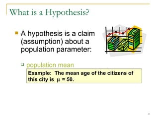
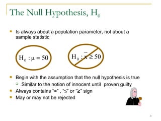
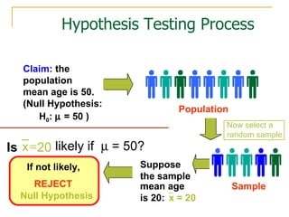
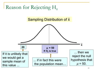
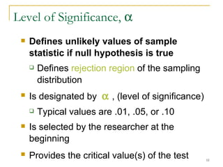
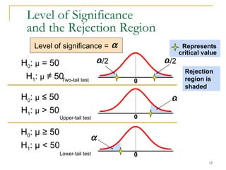
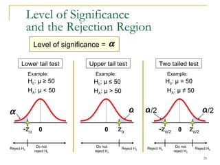
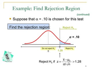
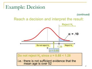
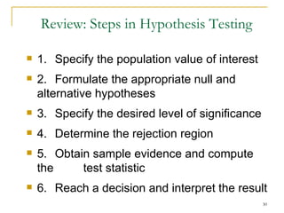
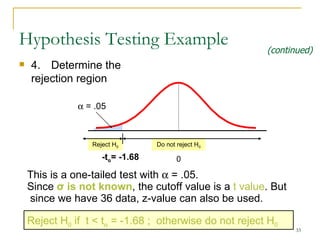
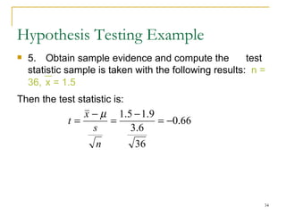
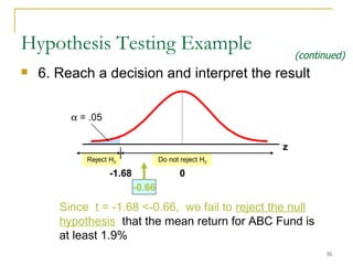
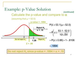
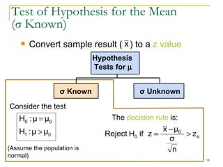
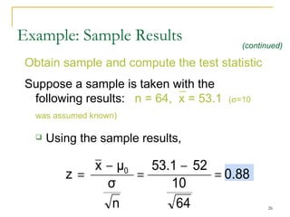
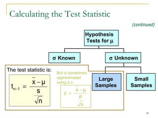
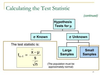
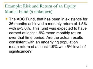
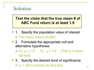
This document provides an introduction to hypothesis testing, including: 1. Defining hypotheses as claims about population parameters and the distinction between the null and alternative hypotheses. 2. Explaining the hypothesis testing process, including specifying the significance level, determining the rejection region, calculating test statistics, and making a decision. 3. Providing examples of one-sample z-tests and t-tests for the mean when the population standard deviation is known and unknown. 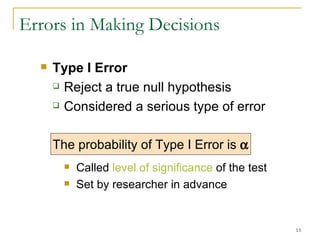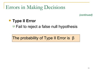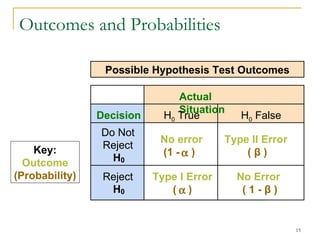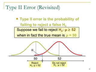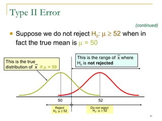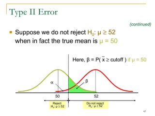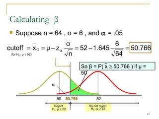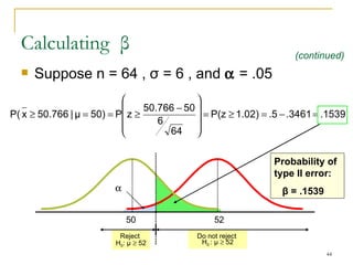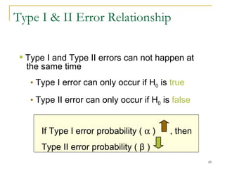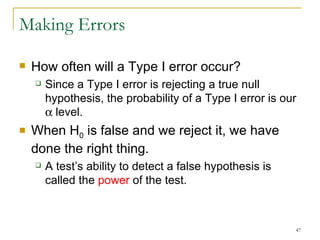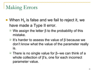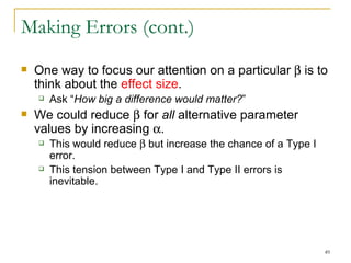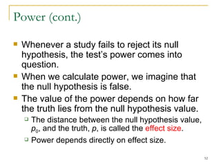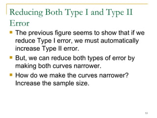4. Discussing type I and type II errors and how significance levels influence the probability of each.

1. Introduction to Hypothesis Testing Istanbul Bilgi University FEC 512 Financial Econometrics-I Asst. Prof. Dr. Orhan Erdem

2. What is a Hypothesis? A hypothesis is a claim (assumption) about a population parameter: population mean Example: The mean age of the citizens of this city is  = 50.

3. Is always about a population parameter, not about a sample statistic Begin with the assumption that the null hypothesis is true Similar to the notion of innocent until proven guilty Always contains “=” , “≤” or “  ” sign May or may not be rejected The Null Hypothesis, H 0

4. The Alternative Hypothesis, H A Is the opposite of the null hypothesis e.g.: The mean age of this city is not 50 ( H A :   50 ) Never contains the “=” , “≤” or “  ” sign May or may not be accepted Is generally the hypothesis that is believed (or needs to be supported) by the researcher

5. Formulating Hypotheses Example : The average annual income of citizens of this city is claimed to be $65,000 per year. An analyst would like to test this claim. What is the appropriate hypothesis test?

6. Example 1 : The average annual income of city A is claimed to be $65,000 per year. An analyst would like to test this claim. What is the appropriate test? H 0 : µ = 65,000 (income is as claimed) status quo H A : µ ≠ 65,000 (income is different than claimed) The analyst will believe the claim unless sufficient evidence is found to discredit it. Formulating Hypotheses

7. A Trial as a Hypothesis Test Hypothesis testing is very much like a court trial. The null hypothesis is that the defendant is innocent. We then present the evidence—collect data. Then we judge the evidence—”Could these data plausibly have happened by chance if the null hypothesis were true?” If they were very unlikely to have occurred, then the evidence raises more than a reasonable doubt in our minds about the null hypothesis.

8. What to Do with an “Innocent” Defendant If the evidence is not strong enough to reject the presumption of innocent, the jury returns with a verdict of “not guilty.” The jury does not say that the defendant is innocent.All it says is that there is not enough evidence to convict, to reject innocence. The defendant may, in fact, be innocent, but the jury has no way to be sure. Said statistically, we will fail to reject the null hypothesis. We never declare the null hypothesis to be true, because we simply do not know whether it’s true or not.

9. Population Claim: the population mean age is 50. (Null Hypothesis: REJECT Suppose the sample mean age is 20: x = 20 Sample Null Hypothesis 20 likely if  = 50?  Is Hypothesis Testing Process If not likely, Now select a random sample H 0 :  = 50 ) x

10. Reason for Rejecting H 0 Sampling Distribution of x  = 50 If H 0 is true If it is unlikely that we would get a sample mean of this value ... ... then we reject the null hypothesis that  = 50. 20 ... if in fact this were the population mean… x

11. Level of Significance,  Defines unlikely values of sample statistic if null hypothesis is true Defines rejection region of the sampling distribution Is designated by  , (level of significance) Typical values are .01, .05, or .10 Is selected by the researcher at the beginning Provides the critical value(s) of the test

12. Level of Significance and the Rejection Region H 0 : μ ≥ 50 H 1 : μ < 50 0 H 0 : μ ≤ 50 H 1 : μ > 50   Represents critical value Lower-tail test Level of significance =  0 Upper-tail test Two-tail test Rejection region is shaded /2 0  /2  H 0 : μ = 50 H 1 : μ ≠ 50

13. Errors in Making Decisions Type I Error Reject a true null hypothesis Considered a serious type of error The probability of Type I Error is  Called level of significance of the test Set by researcher in advance

14. Errors in Making Decisions Type II Error Fail to reject a false null hypothesis The probability of Type II Error is β (continued)

15. Outcomes and Probabilities Actual Situation Decision Do Not Reject H 0 No error (1 - )  Type II Error ( β ) Reject H 0 Type I Error ( )  Possible Hypothesis Test Outcomes H 0 False H 0 True Key: Outcome (Probability) No Error ( 1 - β )

16. Power of the Test The power of a test is the probability of rejecting a null hypothesis that is false i.e., Power = P(Reject H 0 | H 1 is true) Power of the test increases as the sample size increases

17. Hypothesis Tests for the Mean Assume first that the population standard deviation σ is known σ Known σ Unknown Hypothesis Tests for 

18. Test of Hypothesis f or the Mean ( σ Known) Convert sample result ( ) to a z value The decision rule is: σ Known σ Unknown Hypothesis Tests for  Consider the test (Assume the population is normal)

19. Level of Significance and the Rejection Region H 0 : μ ≥ 50 H A : μ < 50 50 H 0 : μ ≤ 50 H A : μ > 50 H 0 : μ = 50 H A : μ ≠ 50   /2 Lower tail test Level of significance =  50 /2  Upper tail test Two tailed test 5 0  - ? ? - ? ? Reject H 0 Reject H 0 Reject H 0 Reject H 0 Do not reject H 0 Do not reject H 0 Do not reject H 0 Example: Example: Example:

20. Level of Significance and the Rejection Region H 0 : μ ≥ 50 H A : μ < 50 0 H 0 : μ ≤ 50 H A : μ > 50 H 0 : μ = 50 H A : μ ≠ 50   /2 Lower tail test Level of significance =  0 /2  Upper tail test Two tailed test 0  -z α z α -z α /2 z α /2 Reject H 0 Reject H 0 Reject H 0 Reject H 0 Do not reject H 0 Do not reject H 0 Do not reject H 0 Example: Example: Example:

21. Upper Tail Tests Reject H 0 Do not reject H 0  z α 0 μ 0 H 0 : μ ≤ μ 0 H 1 : μ > μ 0 Critical value Z Alternate rule:

22. Lower Tail Tests Reject H 0 Do not reject H 0 The cutoff value, or , is called a critical value  -z α x α - z α x α 0 μ H 0 : μ ≥ μ 0 H A : μ < μ 0 I always find a corresponding z value to x

23. Two Tailed Tests There are two cutoff values ( critical values ): or Do not reject H 0 Reject H 0 Reject H 0  /2 -z α /2 x α /2 ± z α /2 x α /2 0 μ 0 H 0 : μ = μ 0 H A : μ  μ 0 z α /2 x α /2 Lower Upper x α /2 Lower Upper  /2

24. Example: Upper-Tail Z Test for Mean (  Known) A supermarket chain manager thinks that customer age have increased, and now average over 52. The company wishes to test this claim. (Assume  = 10 is known) H 0 : μ ≤ 52 the average is not over 52 per month H 1 : μ > 52 the average is greater than 52 (i.e., sufficient evidence exists to support the manager’s claim) Form hypothesis test:

25. Suppose that  = .10 is chosen for this test Find the rejection region: Reject H 0 Do not reject H 0  = .10 1.28 0 Reject H 0 Example: Find Rejection Region (continued)

26. Obtain sample and compute the test statistic Suppose a sample is taken with the following results: n = 64, x = 53.1 (  =10 was assumed known) Using the sample results, Example: Sample Results (continued)

27. Example: Decision Reach a decision and interpret the result: Reject H 0 Do not reject H 0   = .10 1.28 0 Reject H 0 Do not reject H 0 since z = 0.88 < 1.28 i.e.: there is not sufficient evidence that the mean age is over 52 z = 0.88 (continued)

28. Calculating the Test Statistic  Known Large Samples  Unknown Hypothesis Tests for  Small Samples The test statistic is: But is sometimes approximated using a z: (continued)

29. Calculating the Test Statistic  Known Large Samples  Unknown Hypothesis Tests for  Small Samples The test statistic is: (The population must be approximately normal) (continued)

30. Review: Steps in Hypothesis Testing 1. Specify the population value of interest 2. Formulate the appropriate null and alternative hypotheses 3. Specify the desired level of significance 4. Determine the rejection region 5. Obtain sample evidence and compute the test statistic 6. Reach a decision and interpret the result

31. Example: Risk and Return of an Equity Mutual Fund ( σ unknown) The ABC Fund, that has been in existence for 36 months achieved a monthly return of 1.5% with s =3.6%. This fund was expected to have earned at least 1.9% mean monthly return over that time period. Are the actual results consistent with an underlying population mean return of at least 1.9% with 5% level of significance?

32. Solution Test the claim that the true mean # of ABC Fund return is at least 1.9 1. Specify the population value of interest The mean return of ABC 2. Formulate the appropriate null and alternative hypotheses H 0 : μ  1.9 H A : μ < 1.9 (This is a lower tail test) 3. Specify the desired level of significance  = .05 is chosen for this test

33. Hypothesis Testing Example 4. Determine the rejection region Reject H 0 Do not reject H 0  = .05 - t α = -1.6 8 0 This is a one-tailed test with  = .05. Since σ is not known , the cutoff value is a t value . But since we have 36 data, z-value can also be used. Reject H 0 if t < t  = -1. 68 ; otherwise do not reject H 0 (continued)

34. 5. Obtain sample evidence and compute the test statistic sample is taken with the following results: n = 36 , x = 1.5 Then the test statistic is: Hypothesis Testing Example

35. 6. Reach a decision and interpret the result Hypothesis Testing Example Reject H 0 Do not reject H 0  = .05 -1. 68 0 -0 . 66 Since t = -1.6 8 <-0.66 , we fail to reject the null hypothesis that the mean return for ABC Fund is at least 1.9% (continued) z

36. Smallest value of  for which H 0 can be rejected Obtain the p-value from a table or computer Compare the p-value with  If p-value <  , reject H 0 If p-value   , do not reject H 0 p-Value Approach to Testing

37. Calculate the p-value and compare to  (assuming that μ = 52.0) Example: p-Value Solution Reject H 0   = .10 Do not reject H 0 1.28 0 Reject H 0 Z = .88 (continued) p-value = .1894 Do not reject H 0 since p-value = .1894 >  = .10

38. p-value example Example: How likely is it to see a sample mean of 0.93 (or something further below the mean) if the true mean is  = 1 . 9 ? p-value = 0.26  = .05 -1.68 -0.66 x

39. Compare the p-value with  If p-value <  , reject H 0 If p-value   , do not reject H 0 p-value example Here: p-value = 0.26  = .05 Since .05 < 0.26 , we fail to reject the null hypothesis (continued)

40. Type II Error (Revisited) Type II error is the probability of failing to reject a false H 0 Reject H 0 : μ  52 Do not reject H 0 : μ  52 52 50 Suppose we fail to reject H 0 : μ  52 when in fact the true mean is μ = 50 

41. Type II Error Suppose we do not reject H 0 :   52 when in fact the true mean is  = 50 Reject H 0 :   52 Do not reject H 0 :   52 52 50 This is the true distribution of x if  = 50 This is the range of x where H 0 is not rejected (continued)

42. Type II Error Suppose we do not reject H 0 : μ  52 when in fact the true mean is μ = 50 Reject H 0 : μ  52 Do not reject H 0 : μ  52  52 50 β Here, β = P( x  cutoff ) if μ = 50 (continued)

43. Suppose n = 64 , σ = 6 , and  = .05 Calculating β Reject H 0 : μ  52 Do not reject H 0 : μ  52  52 50 So β = P( x  50.766 ) if μ = 50 (for H 0 : μ  52) 50.766

44. Suppose n = 64 , σ = 6 , and  = .05 Calculating β Reject H 0 : μ  52 Do not reject H 0 : μ  52  52 50 (continued) Probability of type II error: β = .1539

45. Type I & II Error Relationship Type I and Type II errors can not happen at the same time Type I error can only occur if H 0 is true Type II error can only occur if H 0 is false If Type I error probability (  ) , then Type II error probability ( β )

46. Factors Affecting Type II Error All else equal, β when the difference between hypothesized parameter and its true value β when  β when σ β when n

47. Making Errors How often will a Type I error occur? Since a Type I error is rejecting a true null hypothesis, the probability of a Type I error is our  level. When H 0 is false and we reject it, we have done the right thing. A test’s ability to detect a false hypothesis is called the power of the test.

48. Making Errors When H 0 is false and we fail to reject it, we have made a Type II error. We assign the letter  to the probability of this mistake. It’s harder to assess the value of  because we don’t know what the value of the parameter really is. There is no single value for  --we can think of a whole collection of  ’s, one for each incorrect parameter value.

49. Making Errors (cont.) One way to focus our attention on a particular  is to think about the effect size . Ask “ How big a difference would matter? ” We could reduce  for all alternative parameter values by increasing  . This would reduce  but increase the chance of a Type I error. This tension between Type I and Type II errors is inevitable .

50. Power The power of a test is the probability that it correctly rejects a false null hypothesis. When the power is high, we can be confident that we’ve looked hard enough at the situation. The power of a test is 1 –  .

51. Type II Error Suppose we do not reject H 0 : μ  52 when in fact the true mean is μ = 50 Reject H 0 : μ  52 Do not reject H 0 : μ  52  52 50 β (continued) Power

52. Power (cont.) Whenever a study fails to reject its null hypothesis, the test’s power comes into question. When we calculate power, we imagine that the null hypothesis is false. The value of the power depends on how far the truth lies from the null hypothesis value. The distance between the null hypothesis value, p 0 , and the truth, p , is called the effect size . Power depends directly on effect size.

53. Reducing Both Type I and Type II Error The previous figure seems to show that if we reduce Type I error, we must automatically increase Type II error. But, we can reduce both types of error by making both curves narrower. How do we make the curves narrower? Increase the sample size.