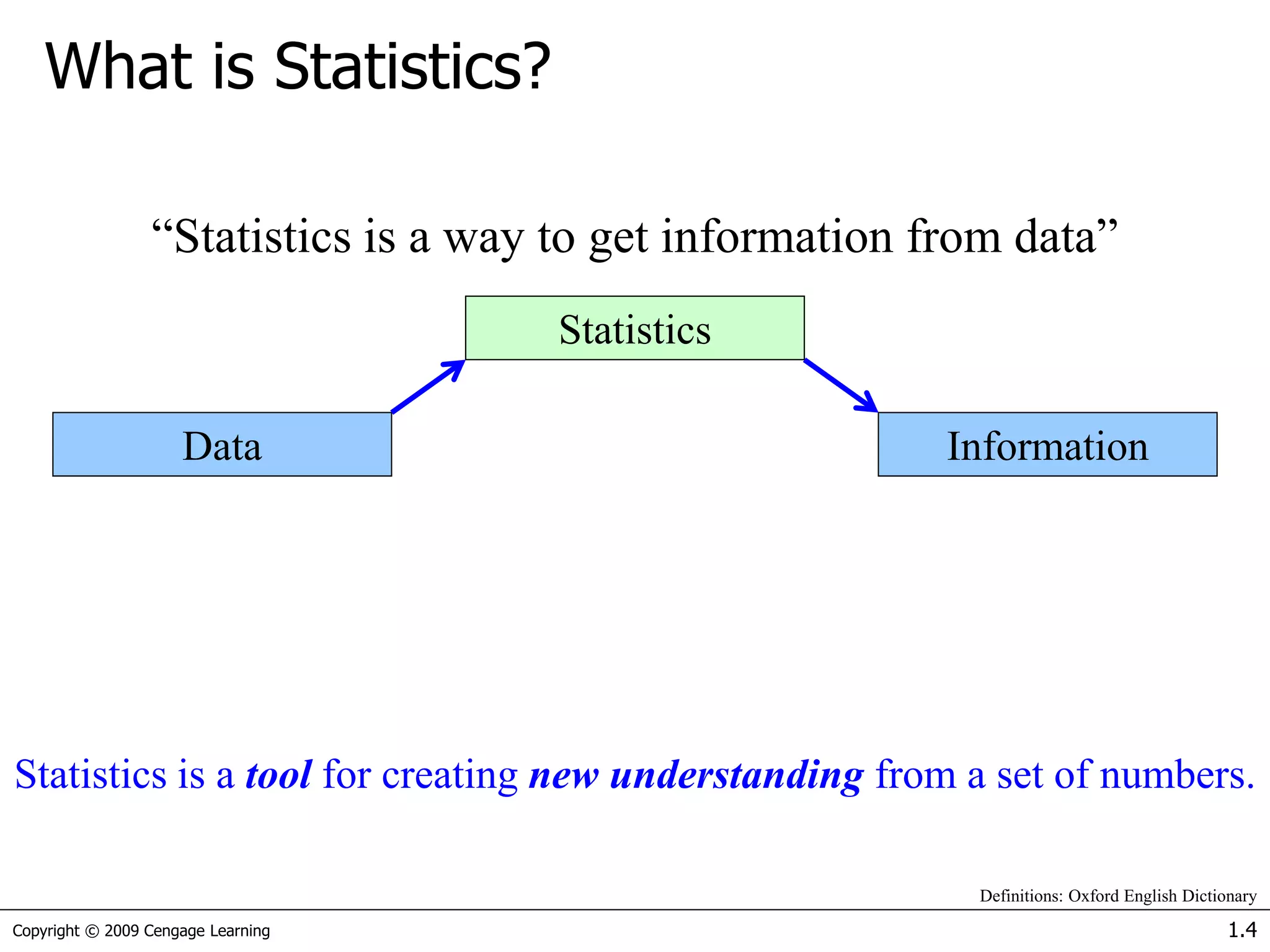
This document provides an introduction to basic statistical concepts. It defines statistics as a tool for extracting information from data. Key concepts discussed include:
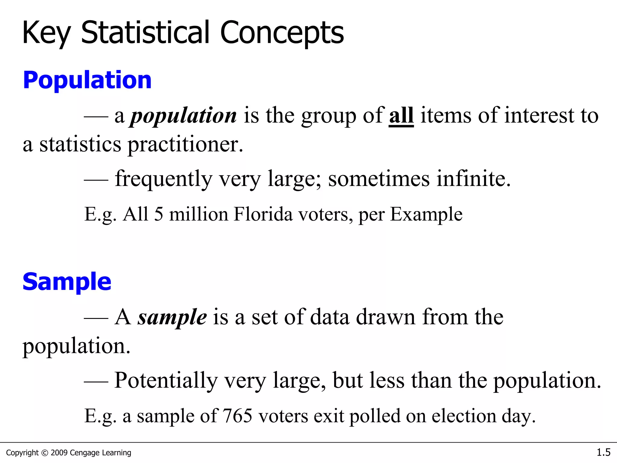
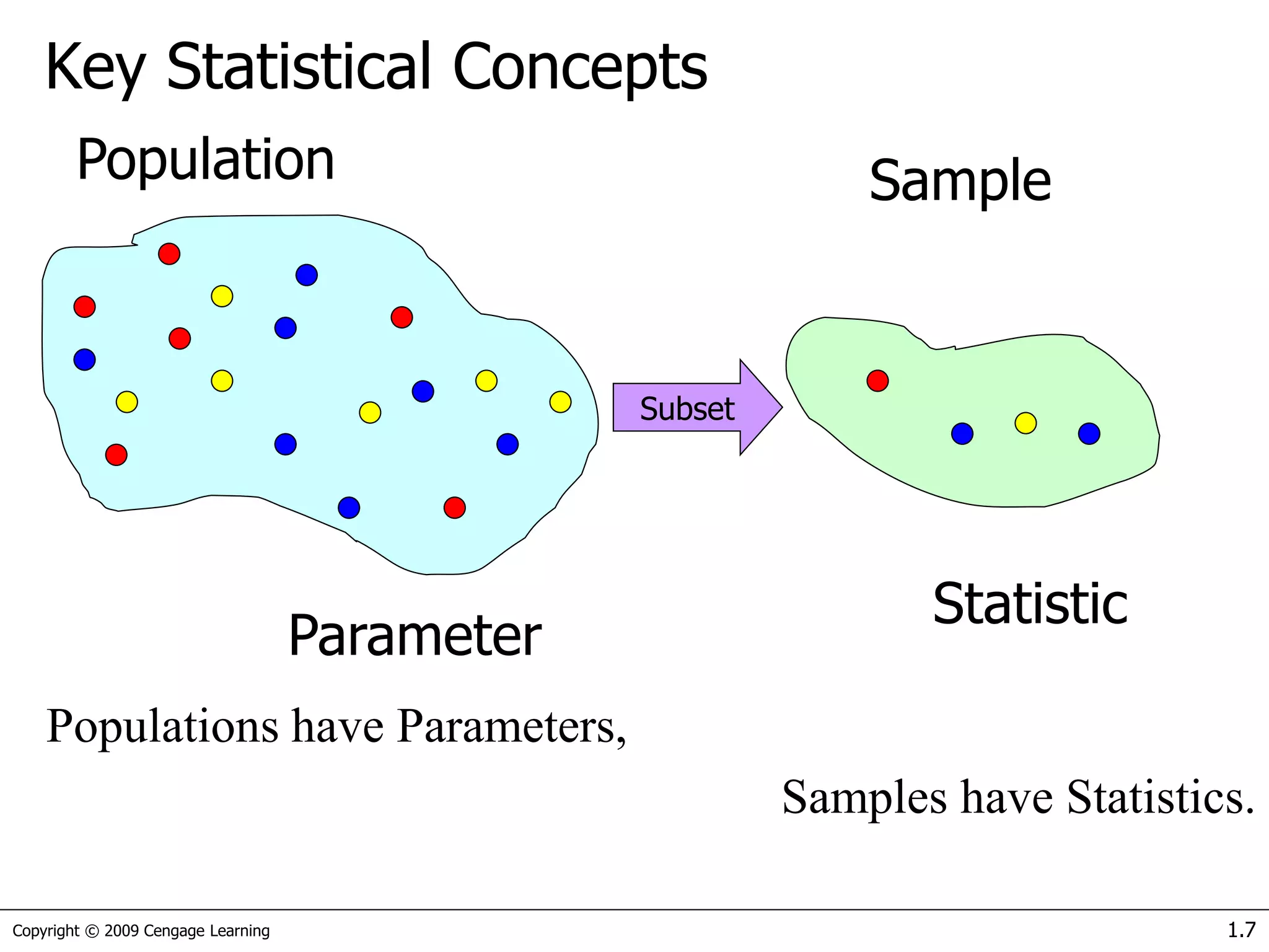
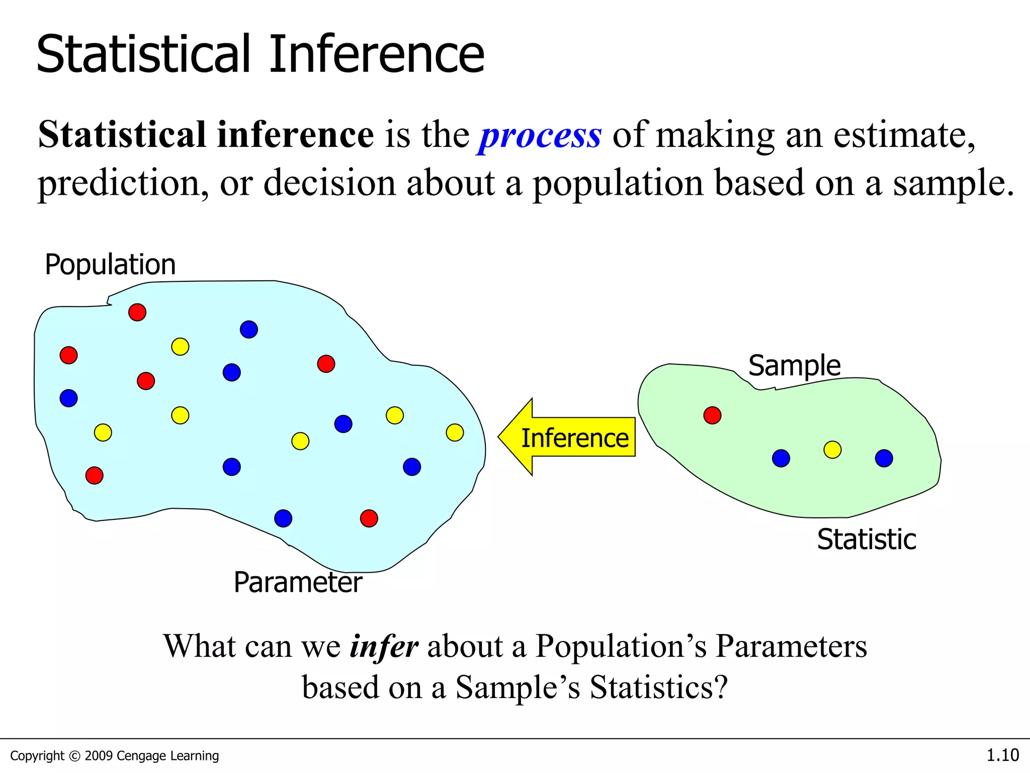
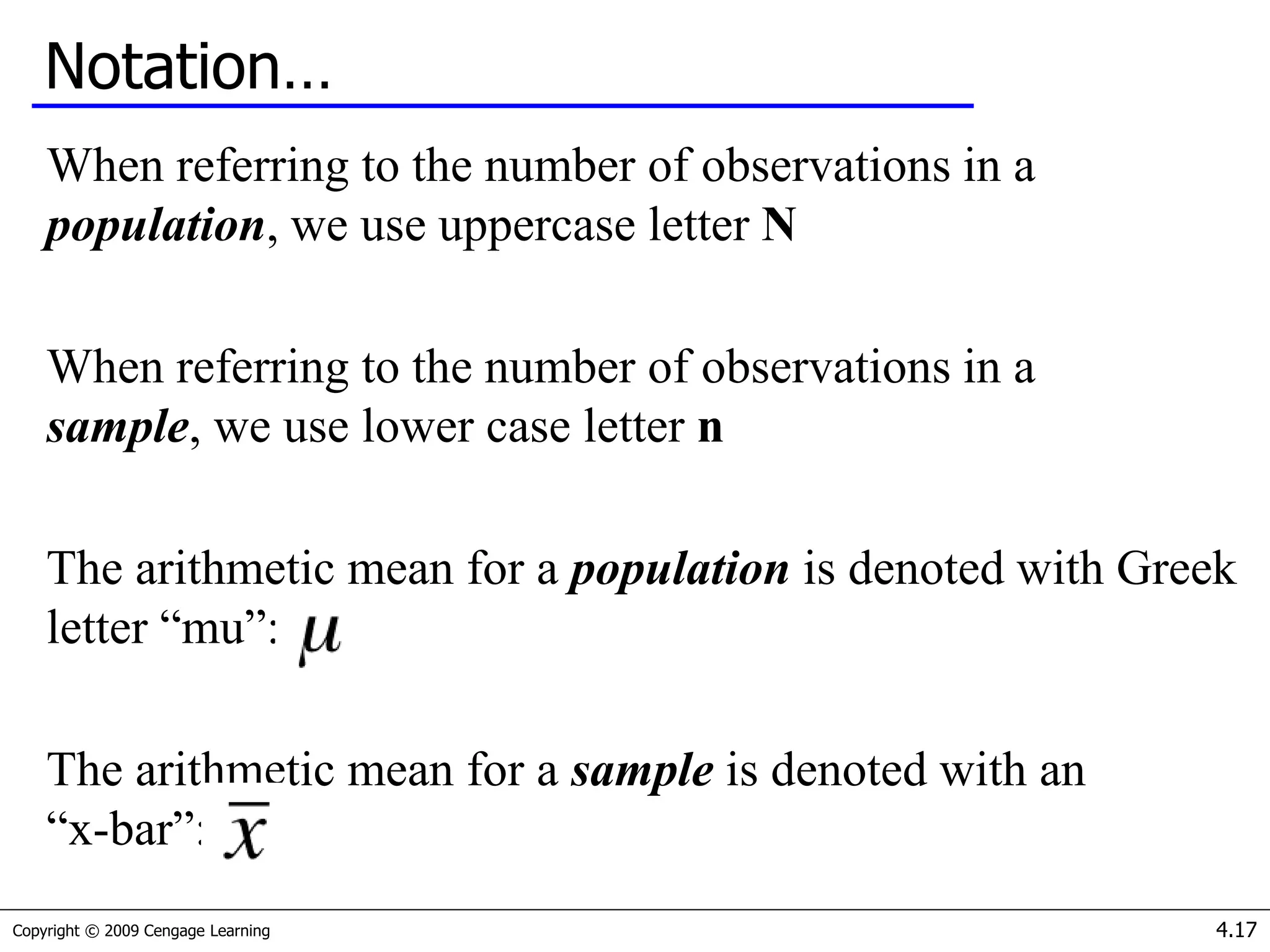
- Population and sample - A population is the whole group being studied, a sample is a subset of the population.
- Parameter and statistic - Parameters describe populations, statistics describe samples.
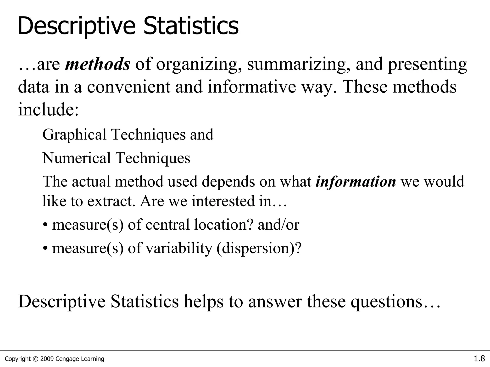
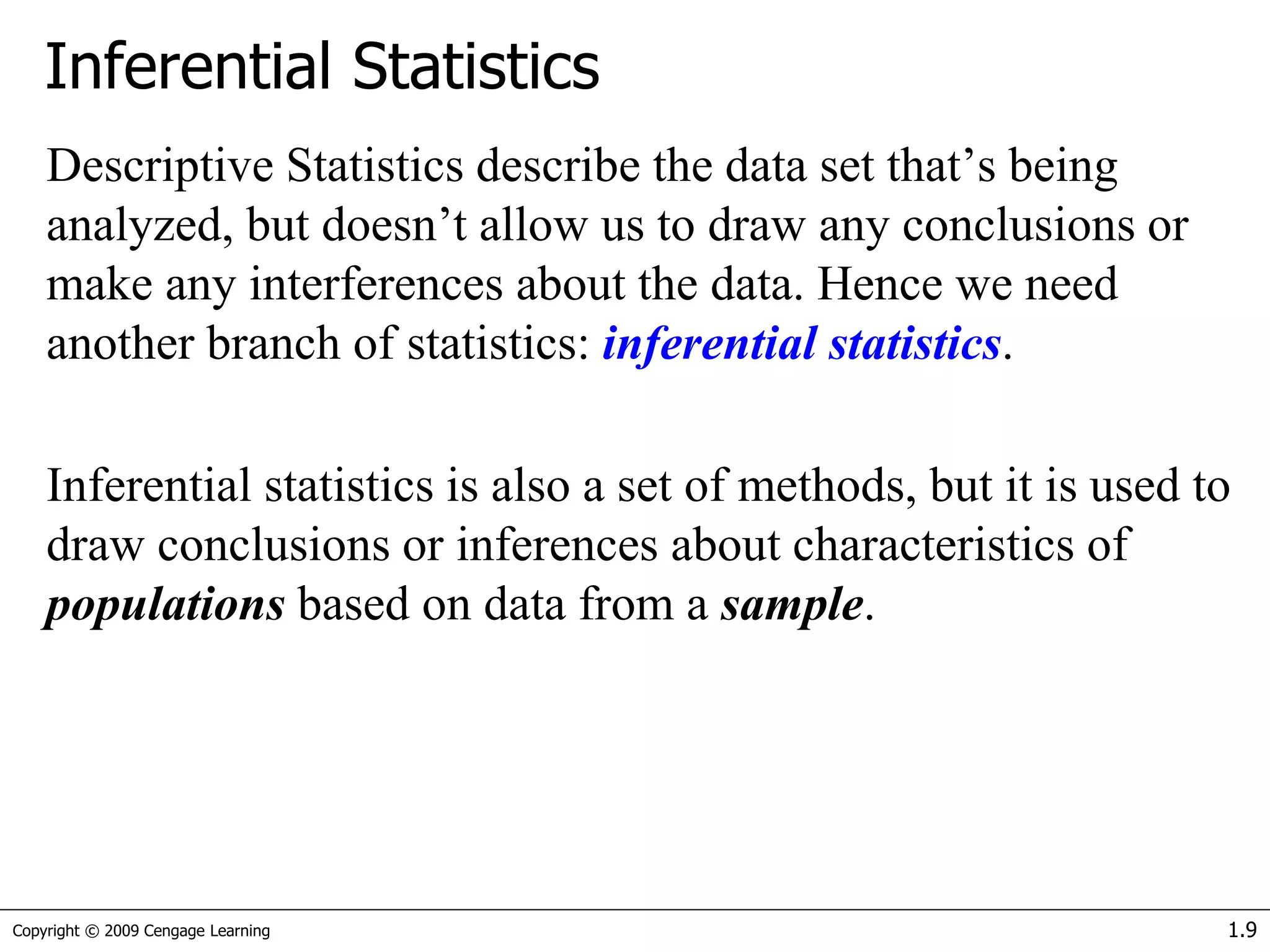
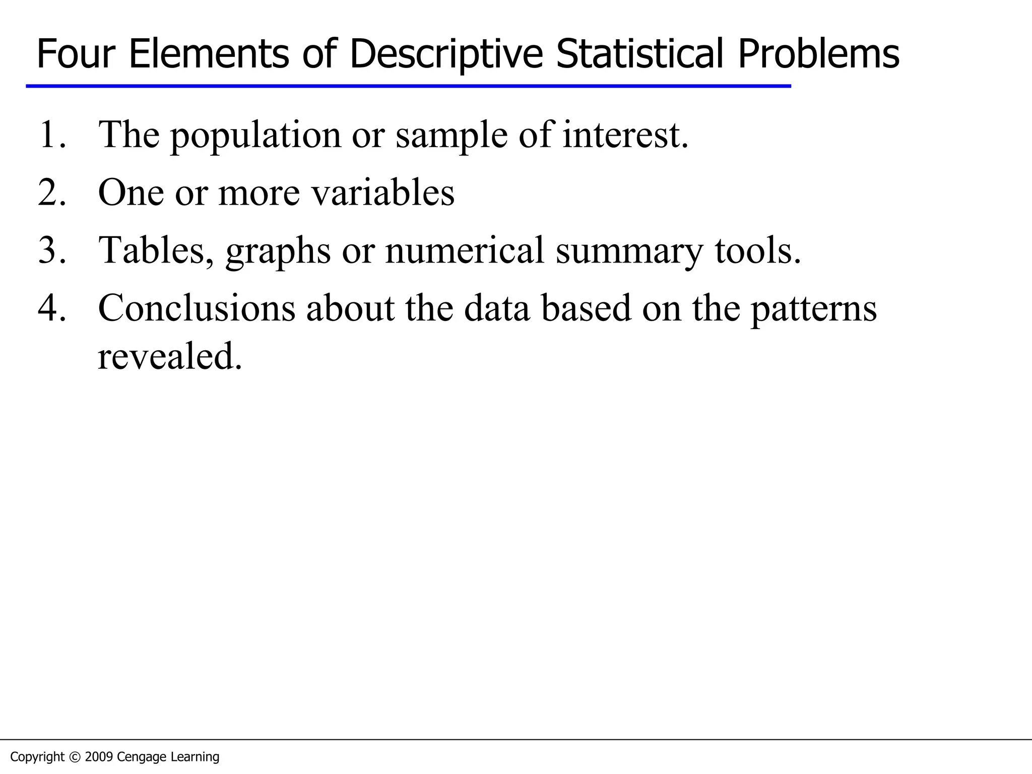
- Descriptive and inferential statistics - Descriptive statistics summarize and organize data, inferential statistics make inferences about populations from samples.
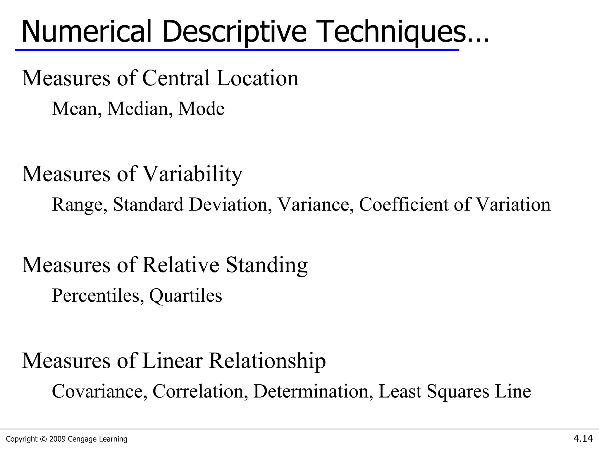
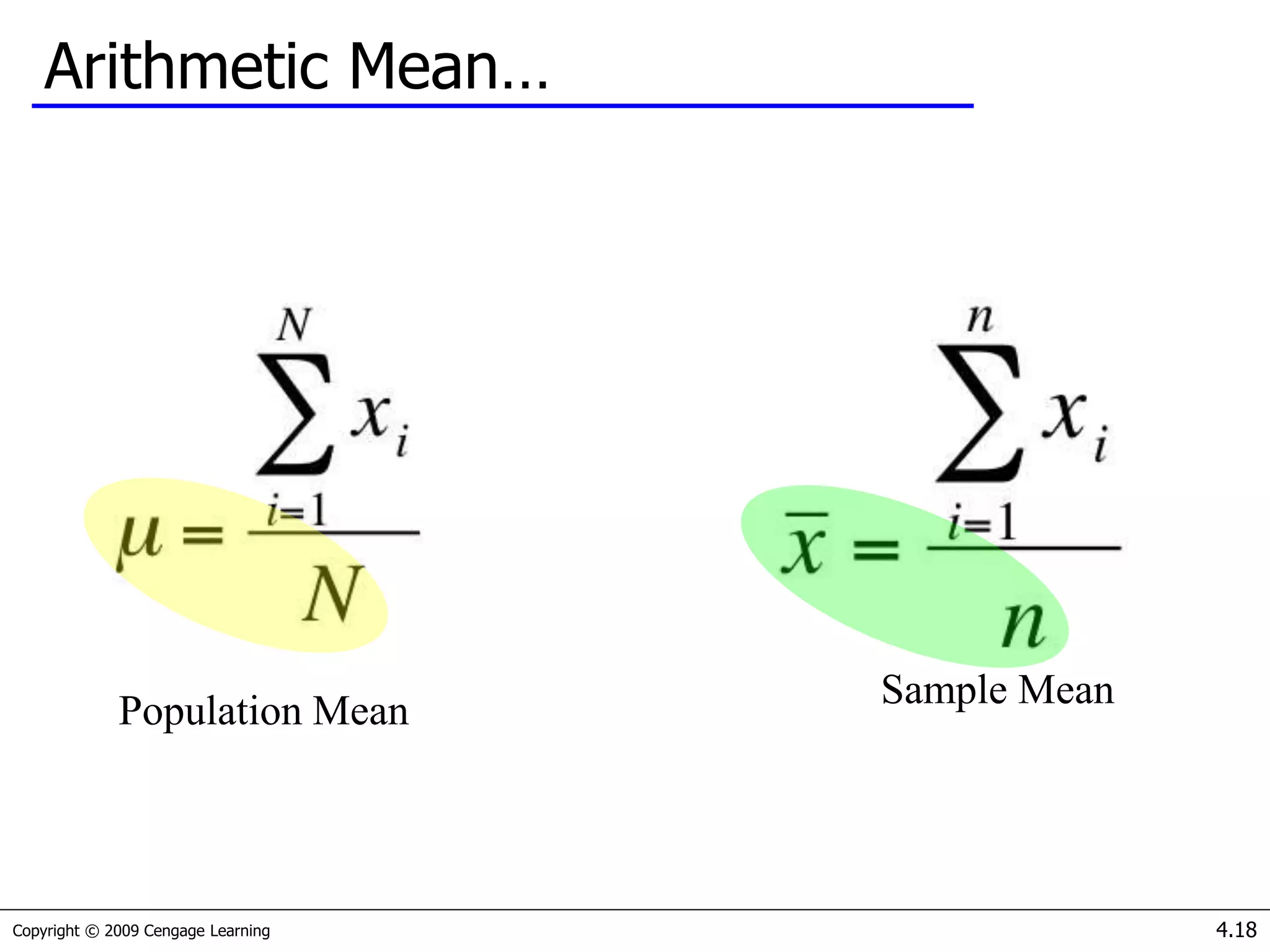
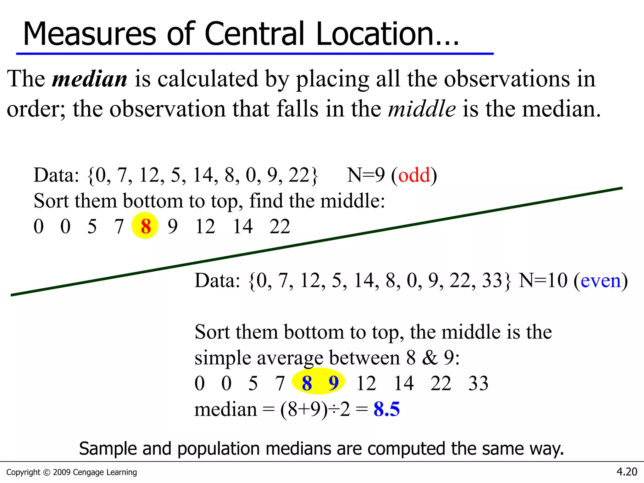
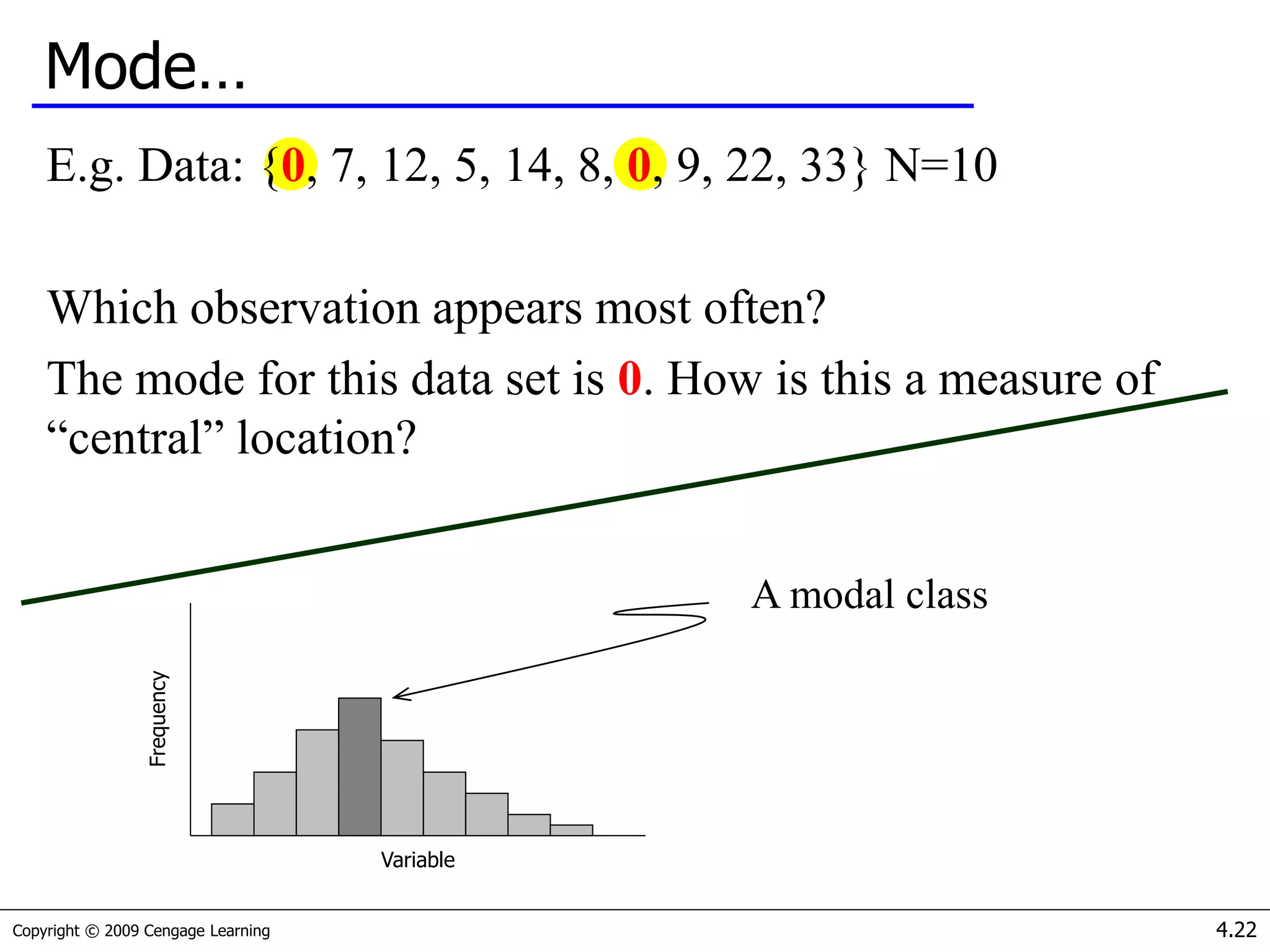
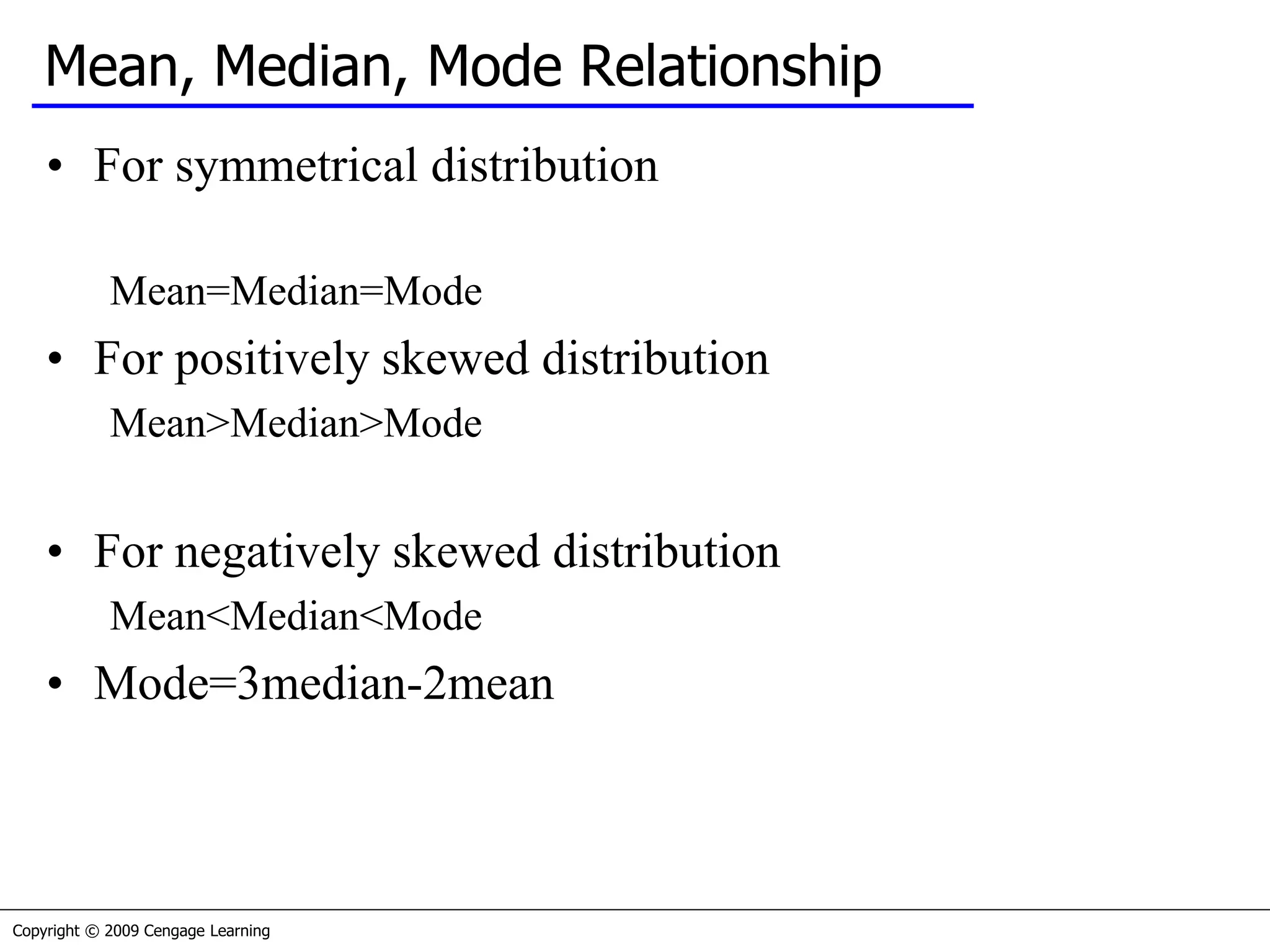
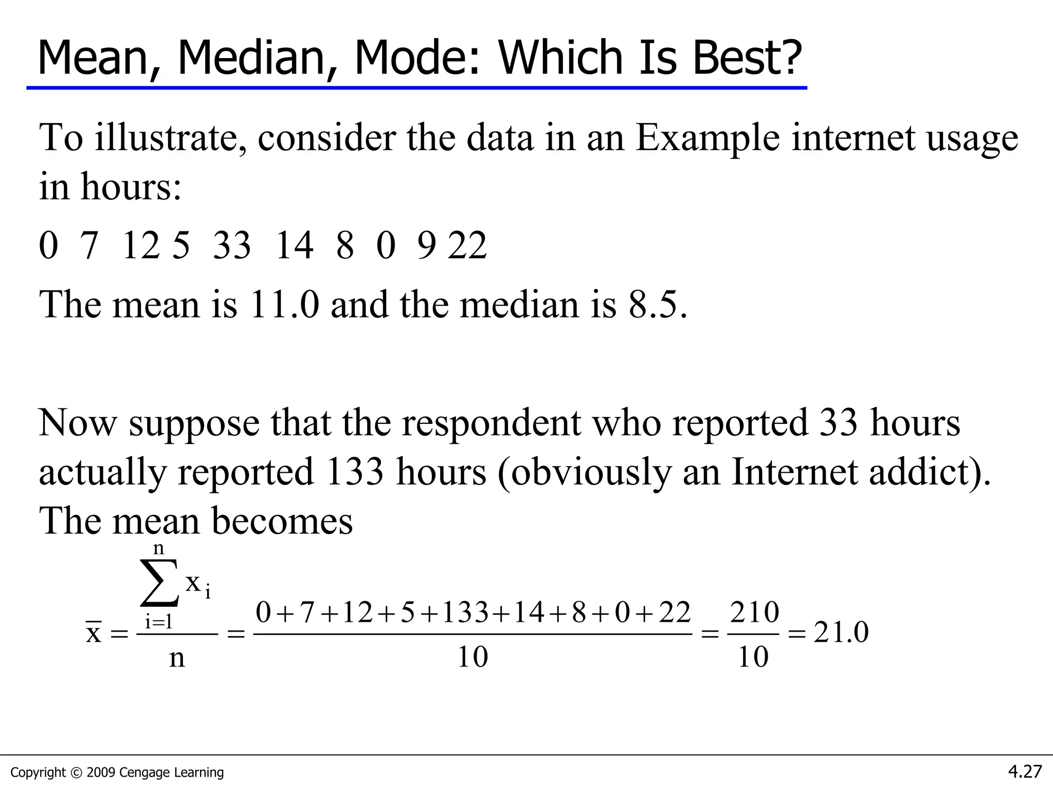
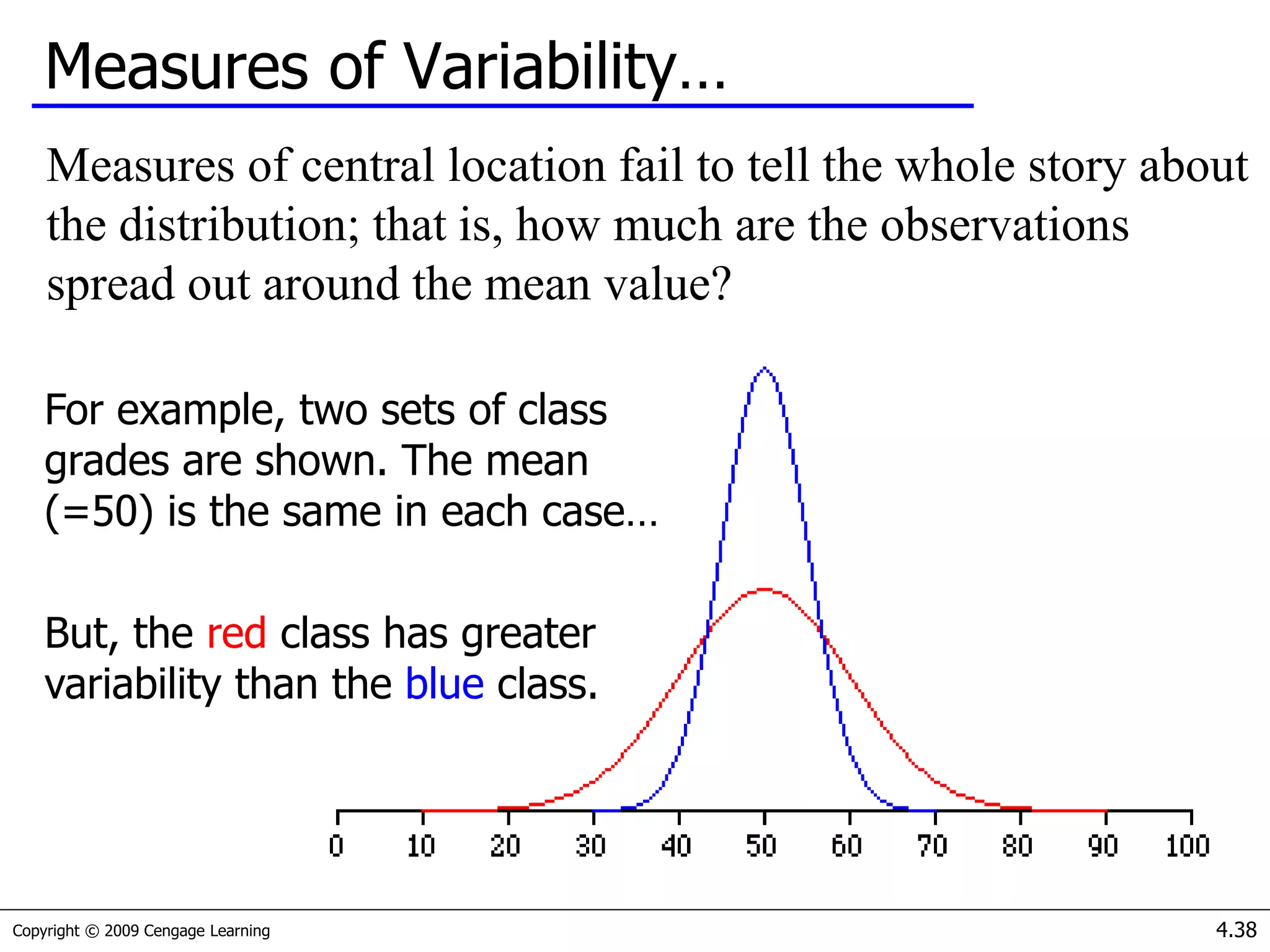
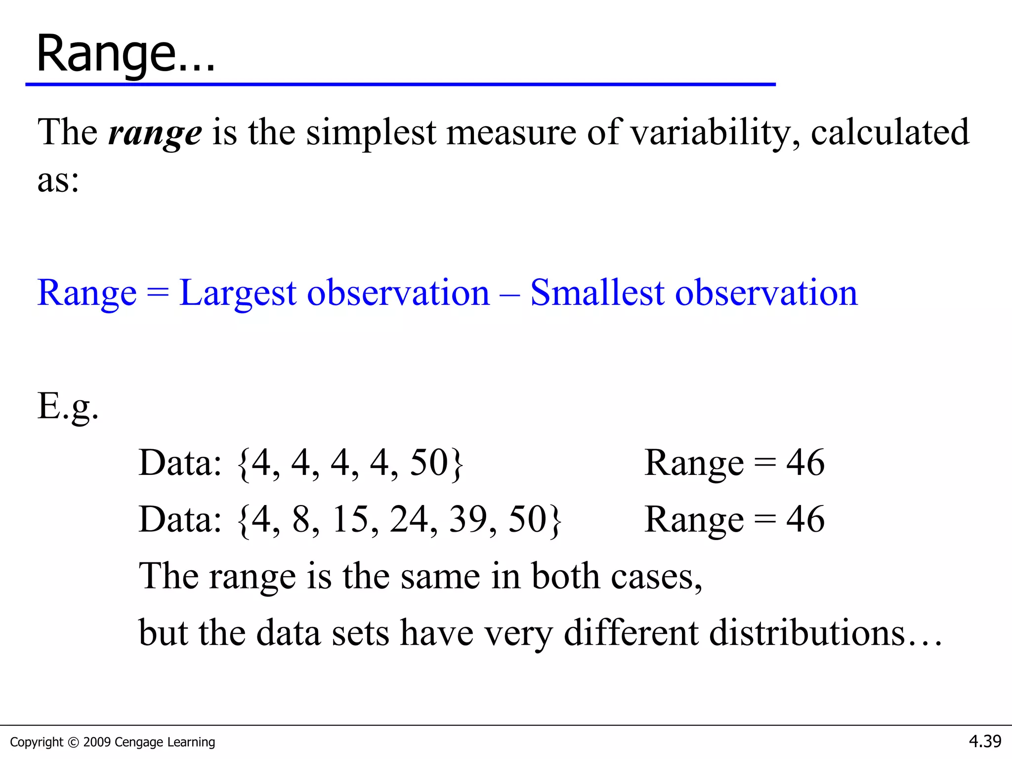
- Measures of central tendency (mean, median, mode) and how to determine which to use based on the data.


![Copyright © 2009 Cengage Learning 4.35
Geometric Mean
The geometric mean of our investment illustration is
The geometric mean is therefore 0%. This is the single
“average” return that allows us to compute the value of the
investment at the end of the investment period from the
beginning value. Thus, using the formula for compound
interest with the rate = 0%, we find
Value at the end of the investment period = 1,000(1 + Rg)2 =
1,000(1 + 0) 2 = 1,000
1)R1)...(R1)(R1(R n
n21g
0111])50.[1)(11(2 ](https://image.slidesharecdn.com/session1-200320035316/75/Introduction-to-statistics-data-analysis-35-2048.jpg)


![Copyright © 2009 Cengage Learning 4.47
Standard Deviation…
Consider Example 4.8 [Xm04-08]where a golf club manufacturer has
designed a new club and wants to determine if it is hit more
consistently (i.e. with less variability) than with an old club.
Using Data > Data Analysis > Descriptive Statistics in Excel, we
produce the following tables for interpretation…
You get more
consistent
distance with the
new club.](https://image.slidesharecdn.com/session1-200320035316/75/Introduction-to-statistics-data-analysis-47-2048.jpg)


![Copyright © 2009 Cengage Learning 4.80
Example 4.17
A tool and die maker operates out of a small shop making specialized
tools.
He is considering increasing the size of his business and needed to
know more about his costs.
One such cost is electricity, which he needs to operate his machines
and lights. (Some jobs require that he turn on extra bright lights to
illuminate his work.)
He keeps track of his daily electricity costs and the number of tools
that he made that day. Determine the fixed and variable electricity
costs. [Xm04-17]](https://image.slidesharecdn.com/session1-200320035316/75/Introduction-to-statistics-data-analysis-80-2048.jpg)


