Download to read offline
![11/5/2018
7
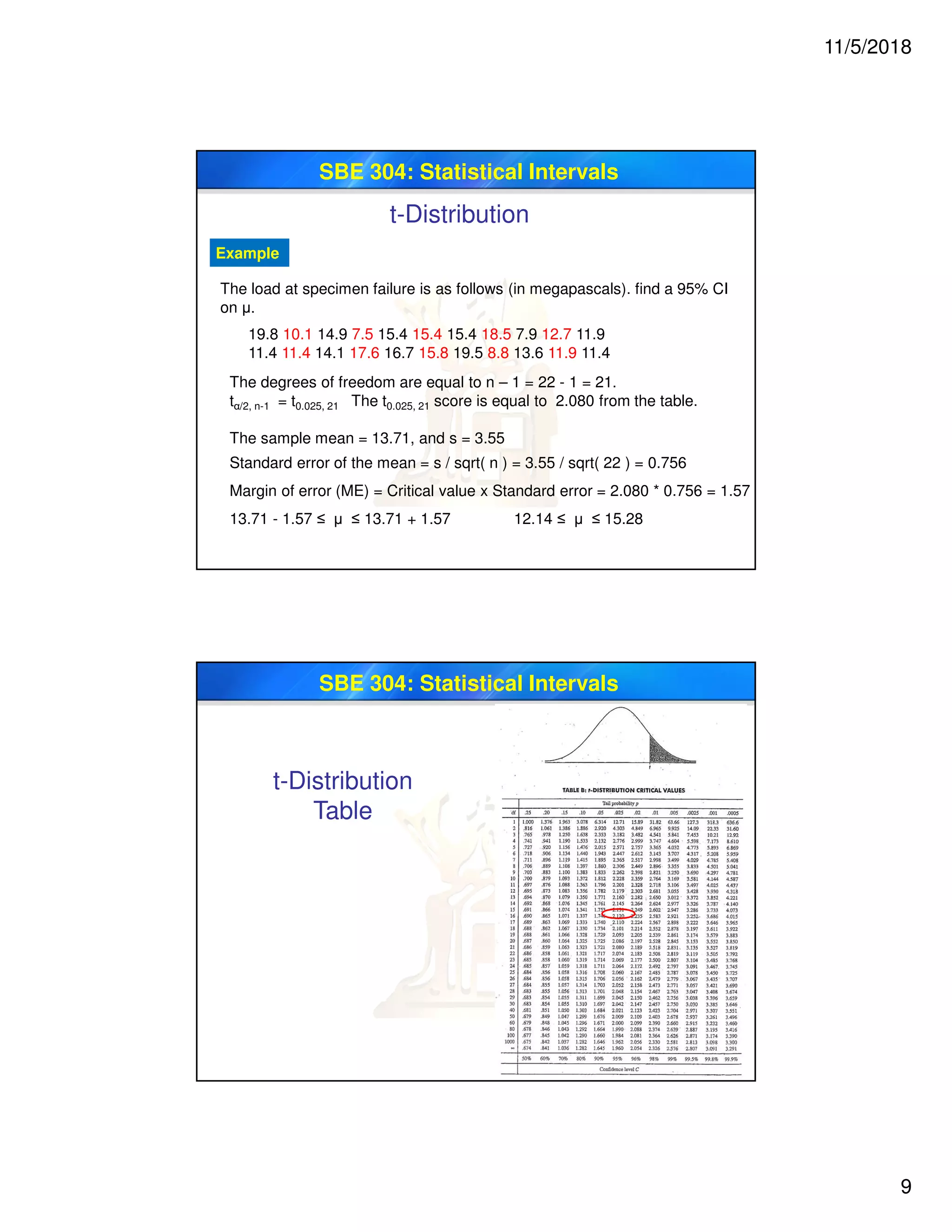
SBE 304: Statistical Intervals
t-Distribution
Student's t-distribution (or simply the t-distribution) is a
continuous probability distribution that arises when
estimating the mean of a normally distributed population in
situations where the sample size is small and/or the
standard deviation of the population σ is unknown. When
either of these problems occur, statisticians rely on the
distribution of the t-statistic whose values are given by:
t = [ x - μ ] / [ s / sqrt( n ) ]
-
(also known as the t score)
where x is the sample mean, μ is the population mean, s is the
standard deviation of the sample, and n is the sample size.
-
SBE 304: Statistical Intervals
Degrees of Freedom
The particular form of the t distribution is determined by its
degrees of freedom. The degrees of freedom refers to the
number of independent observations in a set of data.
The number of independent observations is equal to the sample
size minus one. Hence, the distribution of the t statistic from
samples of size 8 would be described by a t distribution having 8 -
1 or 7 degrees of freedom. Similarly, a t distribution having 15
degrees of freedom would be used with a sample of size 16.
t-Distribution](https://image.slidesharecdn.com/lec5statisticalintervals-200125203037/75/Lec-5-statistical-intervals-7-2048.jpg)

This document discusses confidence intervals, which are interval estimates of population parameters that indicate the reliability of sample estimates. The document defines confidence intervals and explains how they are constructed. It also discusses point estimates versus interval estimates and describes how to calculate confidence intervals for means, proportions, and when the population standard deviation is unknown using the t-distribution. Examples are provided to illustrate how to construct confidence intervals in different situations.