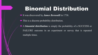
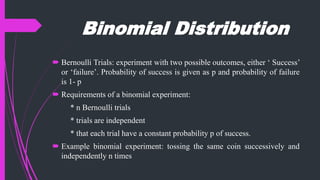
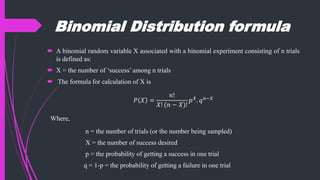
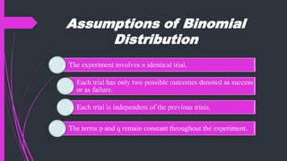
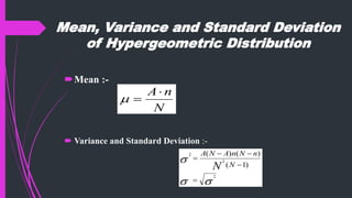
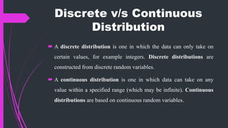
Discrete Distributions:
Binomial, Poisson & Hyper-
geometric
Pooja Yadav,
Research Scholar
Central University of Rajasthan, Ajmer
Satyender Yadav
Research Scholar,
UCCMS, MLSU, Udaipur
Topics Covered
1. Discrete versus continuous distributions
2. Mean, Variance and Standard Deviation
of Discrete Distribution
3. Binomial Distribution
4. Poisson Distribution
5. Hypergeometric Distribution
Discrete & Continuous
Distribution
Discrete distributions:- When the parameter
being measured can only take on certain
values, such as the integers 0, 1 etc. the
probability distribution is called a discrete
distribution. Ex- distribution of the number of
nonconformities or defects in printed circuit
boards would be a discrete distribution
Continuous distributions:- When the variable being
measured is expressed on a continuous scale, its
probability distribution is called a continuous
distribution. Ex- The probability distribution of
metal layer thickness is continuous.
Discrete v/s Continuous
Distribution
 A discrete distribution is one in which the data can only take on
certain values, for example integers. Discrete distributions are
constructed from discrete random variables.
 A continuous distribution is one in which data can take on any
value within a specified range (which may be infinite). Continuous
distributions are based on continuous random variables.
Random Variables
 Random Variable – A random variable is a variable that contains
the outcomes of a chance of experiment.
 A random variable is a discrete random variable if the set of all
possible values is at most a finite or a countably infinite number of
possible values.
 Discrete random variables are usually generated from experiments
in which things are “counted” not “measured”
Example :- If six people are randomly selected from a population and
how many of the six are left-handed is to be determined, the random
variable produced is discrete.
Some Important Terms
Mean- The Mean of a probability distribution is a measure of
the central tendency in the distribution, or its location.
Variance- The scatter, spread, or variability in a distribution is
expressed by the variance.
Standard Deviation- The standard deviation is a measure of
spread or scatter in the population expressed in the original
terms.
Mean, Variance and Standard
Deviation of Discrete Distributions
1. Mean of Discrete Distributions :-
The mean or expected value of a discrete distribution is the long-
run average of occurrences.
Formula
𝜇 = 𝐸 𝑥 = [ 𝑥 ∗ 𝑃(𝑥)]
Where,
E(x) = long-run average
x = an outcome
P(x) = probability of that outcome
Mean, Variance and Standard
Deviation of Discrete Distributions
2. Variance and Standard Deviation of a Discrete Distributions :
 The variance and standard deviation of a discrete distribution are
solved by using the outcomes (x) and probabilities of outcomes [P(x)]
in a manner similar to that of computing a mean.
 The computation of variance and standard deviation use the mean of
the discrete distribution.
Mean, Variance and Standard
Deviation of Discrete Distributions
2. Formula of Variance and Standard Deviation of Discrete Distributions :-
 Variance →
𝜎2
= [(𝑥 − 𝜇)2
∗ 𝑃 𝑥 ]
Where,
x = an outcome
P(x) = probability of a given outcome
µ = mean
 Standard Deviation →
𝜎 = [(𝑥 − 𝜇)2 ∗ 𝑃 𝑥 ]
Binomial Distribution
 It was discovered by James Bernoulli in 1738.
 This is a discrete probability distribution.
 A binomial distribution is simply the probability of a SUCCESS or
FAILURE outcome in an experiment or survey that is repeated
multiple times.
Binomial Distribution
 Bernoulli Trials: experiment with two possible outcomes, either ‘ Success’
or ‘failure’. Probability of success is given as p and probability of failure
is 1- p
 Requirements of a binomial experiment:
* n Bernoulli trials
* trials are independent
* that each trial have a constant probability p of success.
 Example binomial experiment: tossing the same coin successively and
independently n times
Binomial Distribution formula
 A binomial random variable X associated with a binomial experiment consisting of n trials
is defined as:
 X = the number of ‘success’ among n trials
 The formula for calculation of X is
𝑃 𝑋 =
𝑛!
𝑋! (𝑛 − 𝑋)!
𝑝 𝑋. 𝑞 𝑛−𝑋
Where,
n = the number of trials (or the number being sampled)
X = the number of success desired
p = the probability of getting a success in one trial
q = 1-p = the probability of getting a failure in one trial
Assumptions of Binomial
Distribution
The experiment involves n identical trial.
Each trial has only two possible outcomes denoted as success
or as failure.
Each trial is independent of the previous trials.
The terms p and q remain constant throughout the experiment.
Mean and Standard Deviation
of a Binomial Distribution
 Mean of Binomial Distribution :-
𝜇 = 𝑛 ∗ 𝑝
 Standard Deviation
𝜎 = 𝑛 ∗ 𝑝 ∗ 𝑞
where,
n = the number of trials (or the number being sampled)
p = the probability of getting a success in one trial
q = 1-p = the probability of getting a failure in one trial
Poisson Distribution
 It was given by Simone – Denis Poisson in 1837.
 Poisson distribution focuses only on the number of discrete
occurrence over some interval or continuum.
 It describes the occurrence of rare events.
 Poisson formula is referred as law of improbable events.
Characteristics of Poisson
Distribution
It is a discrete distribution.
It describes rare events.
Each occurrence is independent of other occurrences.
It describes discrete occurrences over a continuum or
interval.
The occurrences in each interval can range from zero to
infinity.
The expected number of occurrences must hold constant
throughout the experiment.
Poisson Distribution
Conditions to apply the Poisson Probability distribution are:
 1. x is a discrete random variable
 2. The occurrences are random
 3. The occurrences are independent
Useful to model the number of times that a certain event occurs per unit of
time, distance, or volume. Examples of application of Poisson probability
distribution
i) The number of telephone calls received by an office during
ii) The number of defects in a five-foot-long iron rod.
Poisson Distribution Formula
 The probability of x occurrences in an interval is
𝑓 𝑋 = 𝑃 𝑋 = 𝑥 =
𝑒−𝜆 𝜆 𝑥
𝑥!
, 𝑥 = 0,1,2,3, …
Where, 𝜆 is the mean number of occurrences in that interval. ( per unit time
or per unit area)
 Mean and Variance:
𝐸 𝑋 = 𝑉 𝑋 = 𝜆
The mean or expected value of a Poisson distribution is λ (Lambda).
The variance of a Poisson distribution also is λ
The standard deviation of a Poisson distribution is √ λ
Hyper-Geometric Distribution
 Hyper geometric Distribution- An appropriate probability model for
selecting a random sample of n items without replacement from a lot of
N items of which D are nonconforming or defective.
 In these applications, x usually is the class of interest and then that x is
the hyper geometric random variable.
Characteristics of Hypergeometric
Distribution
It is discrete distribution.
Each outcome consists of either a success
or a failure
Sampling is done without replacement
The population, N, is finite and known.
Hyper-geometric Distribution
Formula
 Hypergeomatric distribution applies only to experiments in which the trials are done
without replacements.
 Formula :-
Where,
N = Size of the population
n = sample size
A = number of successes in the population
x = number of success in the sample; sampling is done without replacement
  
P x
C C
C
A x N A n x
N n
( ) 
 
Mean, Variance and Standard Deviation
of Hypergeometric Distribution
Mean :-
 Variance and Standard Deviation :-
N
nA



2
2
2
)1(
)()(




N
nNnANA
N
For any query, doubt and suggestions please mail us at:
pujayadav026@gmail.com
yadavsatyender724@gmail.com

Discrete distributions: Binomial, Poisson & Hypergeometric distributions

  • 1.
    Discrete Distributions: Binomial, Poisson& Hyper- geometric Pooja Yadav, Research Scholar Central University of Rajasthan, Ajmer Satyender Yadav Research Scholar, UCCMS, MLSU, Udaipur
  • 2.
    Topics Covered 1. Discreteversus continuous distributions 2. Mean, Variance and Standard Deviation of Discrete Distribution 3. Binomial Distribution 4. Poisson Distribution 5. Hypergeometric Distribution
  • 3.
    Discrete & Continuous Distribution Discretedistributions:- When the parameter being measured can only take on certain values, such as the integers 0, 1 etc. the probability distribution is called a discrete distribution. Ex- distribution of the number of nonconformities or defects in printed circuit boards would be a discrete distribution Continuous distributions:- When the variable being measured is expressed on a continuous scale, its probability distribution is called a continuous distribution. Ex- The probability distribution of metal layer thickness is continuous.
  • 4.
    Discrete v/s Continuous Distribution A discrete distribution is one in which the data can only take on certain values, for example integers. Discrete distributions are constructed from discrete random variables.  A continuous distribution is one in which data can take on any value within a specified range (which may be infinite). Continuous distributions are based on continuous random variables.
  • 5.
    Random Variables  RandomVariable – A random variable is a variable that contains the outcomes of a chance of experiment.  A random variable is a discrete random variable if the set of all possible values is at most a finite or a countably infinite number of possible values.  Discrete random variables are usually generated from experiments in which things are “counted” not “measured” Example :- If six people are randomly selected from a population and how many of the six are left-handed is to be determined, the random variable produced is discrete.
  • 6.
    Some Important Terms Mean-The Mean of a probability distribution is a measure of the central tendency in the distribution, or its location. Variance- The scatter, spread, or variability in a distribution is expressed by the variance. Standard Deviation- The standard deviation is a measure of spread or scatter in the population expressed in the original terms.
  • 7.
    Mean, Variance andStandard Deviation of Discrete Distributions 1. Mean of Discrete Distributions :- The mean or expected value of a discrete distribution is the long- run average of occurrences. Formula 𝜇 = 𝐸 𝑥 = [ 𝑥 ∗ 𝑃(𝑥)] Where, E(x) = long-run average x = an outcome P(x) = probability of that outcome
  • 8.
    Mean, Variance andStandard Deviation of Discrete Distributions 2. Variance and Standard Deviation of a Discrete Distributions :  The variance and standard deviation of a discrete distribution are solved by using the outcomes (x) and probabilities of outcomes [P(x)] in a manner similar to that of computing a mean.  The computation of variance and standard deviation use the mean of the discrete distribution.
  • 9.
    Mean, Variance andStandard Deviation of Discrete Distributions 2. Formula of Variance and Standard Deviation of Discrete Distributions :-  Variance → 𝜎2 = [(𝑥 − 𝜇)2 ∗ 𝑃 𝑥 ] Where, x = an outcome P(x) = probability of a given outcome µ = mean  Standard Deviation → 𝜎 = [(𝑥 − 𝜇)2 ∗ 𝑃 𝑥 ]
  • 10.
    Binomial Distribution  Itwas discovered by James Bernoulli in 1738.  This is a discrete probability distribution.  A binomial distribution is simply the probability of a SUCCESS or FAILURE outcome in an experiment or survey that is repeated multiple times.
  • 11.
    Binomial Distribution  BernoulliTrials: experiment with two possible outcomes, either ‘ Success’ or ‘failure’. Probability of success is given as p and probability of failure is 1- p  Requirements of a binomial experiment: * n Bernoulli trials * trials are independent * that each trial have a constant probability p of success.  Example binomial experiment: tossing the same coin successively and independently n times
  • 12.
    Binomial Distribution formula A binomial random variable X associated with a binomial experiment consisting of n trials is defined as:  X = the number of ‘success’ among n trials  The formula for calculation of X is 𝑃 𝑋 = 𝑛! 𝑋! (𝑛 − 𝑋)! 𝑝 𝑋. 𝑞 𝑛−𝑋 Where, n = the number of trials (or the number being sampled) X = the number of success desired p = the probability of getting a success in one trial q = 1-p = the probability of getting a failure in one trial
  • 13.
    Assumptions of Binomial Distribution Theexperiment involves n identical trial. Each trial has only two possible outcomes denoted as success or as failure. Each trial is independent of the previous trials. The terms p and q remain constant throughout the experiment.
  • 14.
    Mean and StandardDeviation of a Binomial Distribution  Mean of Binomial Distribution :- 𝜇 = 𝑛 ∗ 𝑝  Standard Deviation 𝜎 = 𝑛 ∗ 𝑝 ∗ 𝑞 where, n = the number of trials (or the number being sampled) p = the probability of getting a success in one trial q = 1-p = the probability of getting a failure in one trial
  • 15.
    Poisson Distribution  Itwas given by Simone – Denis Poisson in 1837.  Poisson distribution focuses only on the number of discrete occurrence over some interval or continuum.  It describes the occurrence of rare events.  Poisson formula is referred as law of improbable events.
  • 16.
    Characteristics of Poisson Distribution Itis a discrete distribution. It describes rare events. Each occurrence is independent of other occurrences. It describes discrete occurrences over a continuum or interval. The occurrences in each interval can range from zero to infinity. The expected number of occurrences must hold constant throughout the experiment.
  • 17.
    Poisson Distribution Conditions toapply the Poisson Probability distribution are:  1. x is a discrete random variable  2. The occurrences are random  3. The occurrences are independent Useful to model the number of times that a certain event occurs per unit of time, distance, or volume. Examples of application of Poisson probability distribution i) The number of telephone calls received by an office during ii) The number of defects in a five-foot-long iron rod.
  • 18.
    Poisson Distribution Formula The probability of x occurrences in an interval is 𝑓 𝑋 = 𝑃 𝑋 = 𝑥 = 𝑒−𝜆 𝜆 𝑥 𝑥! , 𝑥 = 0,1,2,3, … Where, 𝜆 is the mean number of occurrences in that interval. ( per unit time or per unit area)  Mean and Variance: 𝐸 𝑋 = 𝑉 𝑋 = 𝜆 The mean or expected value of a Poisson distribution is λ (Lambda). The variance of a Poisson distribution also is λ The standard deviation of a Poisson distribution is √ λ
  • 19.
    Hyper-Geometric Distribution  Hypergeometric Distribution- An appropriate probability model for selecting a random sample of n items without replacement from a lot of N items of which D are nonconforming or defective.  In these applications, x usually is the class of interest and then that x is the hyper geometric random variable.
  • 20.
    Characteristics of Hypergeometric Distribution Itis discrete distribution. Each outcome consists of either a success or a failure Sampling is done without replacement The population, N, is finite and known.
  • 21.
    Hyper-geometric Distribution Formula  Hypergeomatricdistribution applies only to experiments in which the trials are done without replacements.  Formula :- Where, N = Size of the population n = sample size A = number of successes in the population x = number of success in the sample; sampling is done without replacement    P x C C C A x N A n x N n ( )   
  • 22.
    Mean, Variance andStandard Deviation of Hypergeometric Distribution Mean :-  Variance and Standard Deviation :- N nA    2 2 2 )1( )()(     N nNnANA N
  • 23.
    For any query,doubt and suggestions please mail us at: pujayadav026@gmail.com yadavsatyender724@gmail.com