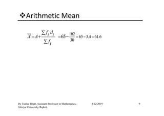
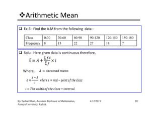
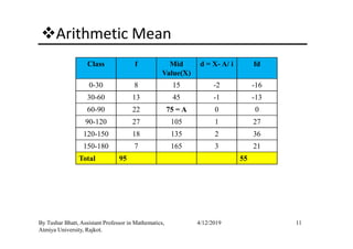
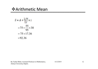
Download to read offline
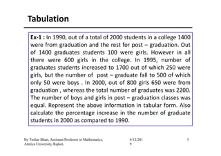
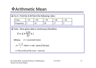
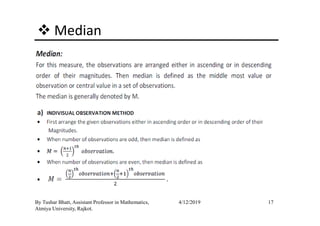
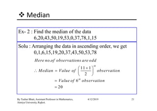
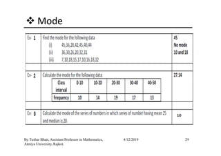
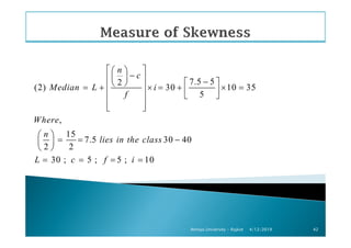
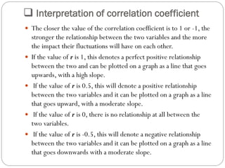
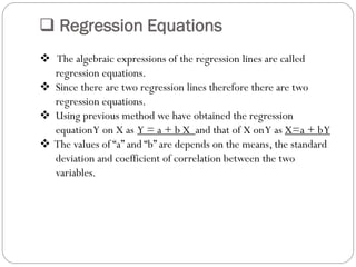
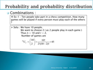
![Graphical Representations of Grouped data
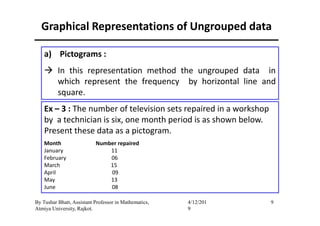
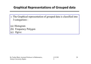
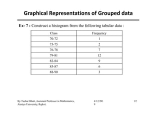
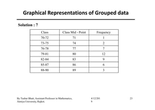
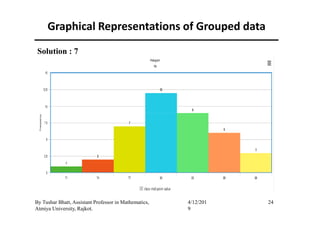
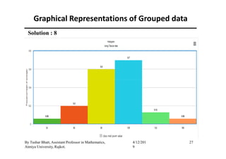
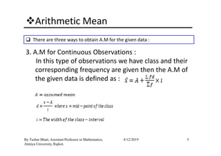
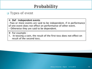
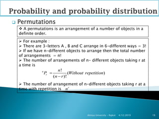
(a) Histogram :
The histogram is mainly used for presentation of grouped data in
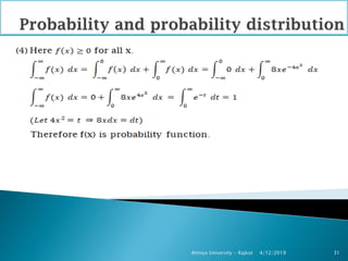
which the respective frequency of the classes are plot on a graph as
a vertical adjacent rectangles.
If class intervals are of equal length then the heights of rectangles
of a histograms are equal to frequencies.
If class intervals are of not equal length then the heights of
21By Tushar Bhatt, Assistant Professor in Mathematics,
Atmiya University, Rajkot.
4/12/201
9
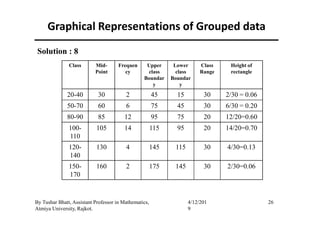
If class intervals are of not equal length then the heights of
rectangles of a histograms are obtain by using following manner:
1. Upper class boundary+5
2. Lower class boundary -5
3. Class range = [(Upper class boundary+5) - (Lower class
boundary -5)]
4. Heights of rectangles are = Frequency of the class / class range.](https://image.slidesharecdn.com/statisticalmethodsform-201021073505/85/Statistical-Methods-21-320.jpg)


![By
Tushar Bhatt
[M.Sc(Maths), M.Phil(Maths), M.Phil(Stat.),M.A(Edu.),P.G.D.C.A]
Assistant Professor in Mathematics,
Atmiya University,
Rajkot
Correlation and Regression](https://image.slidesharecdn.com/statisticalmethodsform-201021073505/85/Statistical-Methods-118-320.jpg)
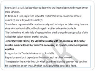


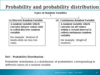
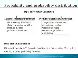
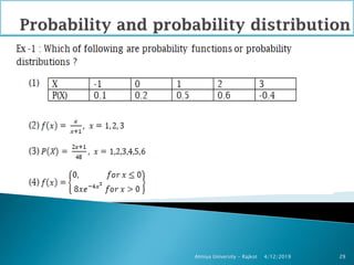
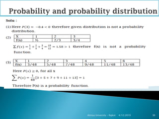

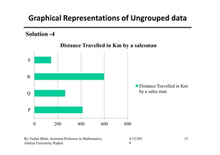
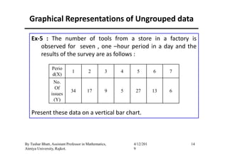
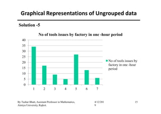
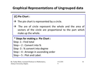
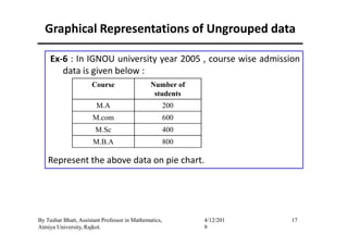
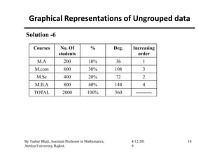
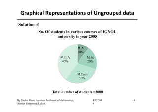
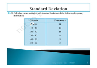
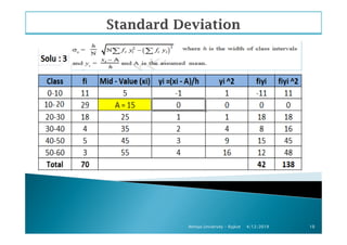
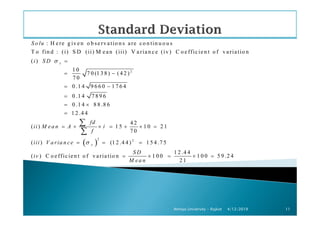
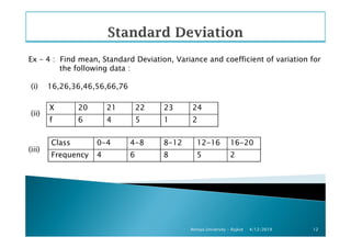
The document outlines a statistics module covering definitions, classifications of data (qualitative, quantitative, temporal, geographical), and data analysis techniques including tabulation and graphical representation methods such as pictograms, bar charts, and pie charts. Examples illustrate how to compile and represent data effectively, analyze trends over time, and construct various types of graphs for both ungrouped and grouped data. Additionally, it touches on measures of central tendency, specifically mean, median, and mode.