Download as PDF, PPTX
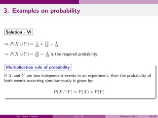
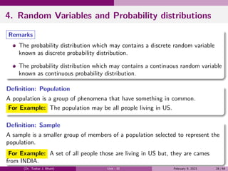
![6. Variance of a Random Variable
Variance is a characteristic of a random variable X and it is used of measure
dispersion (or variation) of X.
If X is a discrete random variable with probability density function f(x), then
expected value of [X − E(X)]2
is called the variance of X and it is denoted
by V (X).
That is V (X) = E[X − E(X)]2
.
If we put E(X) = µ , then V (X) = E(X − µ)2
.
(Dr. Tushar J. Bhatt) Unit - III February 9, 2023 41 / 64](https://image.slidesharecdn.com/unitiiitheoryofprobability1-230306031515-6ff2ea28/85/Theory_of_Probability-pdf-41-320.jpg)
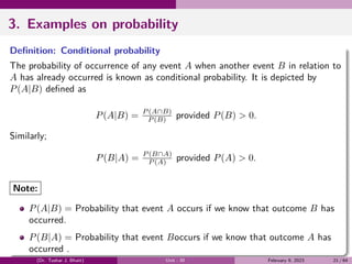
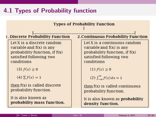
![6.1 Properties of variance
1 V (c) = 0, Where c is a constant.
2 V (cX) = c2
V (x), Where c is a constant.
3 V (X + c) = V (X),Where c is a constant.
4 If X and Y are the independent random variables, then
V (X + Y ) = V (X) + V (Y ).
5 V (X) = E(X2
) − µ2
or V (X) = E(X2
) − [E(X)]2
.
(Dr. Tushar J. Bhatt) Unit - III February 9, 2023 42 / 64](https://image.slidesharecdn.com/unitiiitheoryofprobability1-230306031515-6ff2ea28/85/Theory_of_Probability-pdf-42-320.jpg)
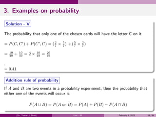
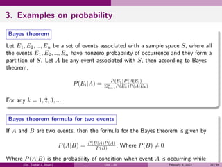
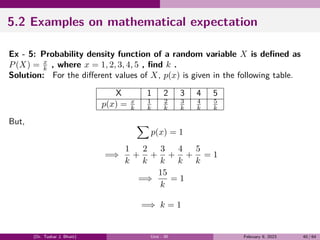
![6.3 Examples on Standard deviation and Variance -
Solution - 1 ...
Form the above table, we have
1 E(X) =
∑
x · p(x) = 0.
2 E(X2
) =
∑
x2
· p(x) = 1.6.
Now V (X) = E(X2
) − [E(X)]2
= 1.6 − 0 = 1.6.
3 E(2x − 3) = 2E(x) − 3 = 2 × 0 − 3 = −3.
4 V (2x − 3) = 22
· V (x) = 4 × 1.6 = 6.4.
(Dr. Tushar J. Bhatt) Unit - III February 9, 2023 45 / 64](https://image.slidesharecdn.com/unitiiitheoryofprobability1-230306031515-6ff2ea28/85/Theory_of_Probability-pdf-45-320.jpg)
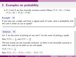
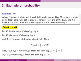
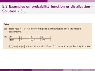
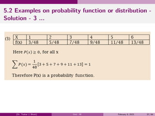
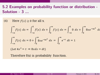
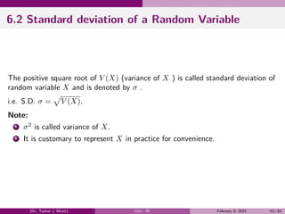
![6.3 Examples on Standard deviation and Variance -
Solution - 2 ...
Form the above table, we have
1 E(X) =
∑
x · p(x) = −1
3 .
2 E(X2
) =
∑
x2
· p(x) = 2
3 .
Now V (X) = E(X2
) − [E(X)]2
= 1.6 − 0 = 1.6.
3 V (X) = E(X2
) − [E(X)]2
= 2
3 −
(
−1
3
)2
= 5
9 .
(Dr. Tushar J. Bhatt) Unit - III February 9, 2023 47 / 64](https://image.slidesharecdn.com/unitiiitheoryofprobability1-230306031515-6ff2ea28/85/Theory_of_Probability-pdf-47-320.jpg)
![6.3 Examples on Standard deviation and Variance
Ex - 3: Mean and S.D. of a random variable X are 5 and 4 respectively.
Find (i) E(X2
) (ii) E(2x + 1)2
(iii) S.D. of V (5 − 3x).
Solution: Here Mean = 5 and S.D. (σ) = 4
∴ E(X) = 5 and V (X) = (S.D. = σ)2
= (4)2
= 16.
1 V (X) = E(X2
) − [E(X)]2
=⇒ 16 = E(X2
) − (5)2
=⇒ E(x2
) = 41.
2 E(2x+1)2
= E(4x2
+4x+1) = 4E(x2
)+4E(x)+1 = 4×41+4×5+1 = 185.
3 V (5 − 3x) = (−3)2
V (x) = 9 × 16 = 144
∴ S.D. of (5 − 3x) =
√
V (5 − 3x) =
√
144 = 12.
(Dr. Tushar J. Bhatt) Unit - III February 9, 2023 48 / 64](https://image.slidesharecdn.com/unitiiitheoryofprobability1-230306031515-6ff2ea28/85/Theory_of_Probability-pdf-48-320.jpg)
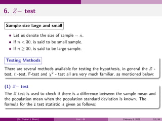
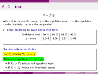
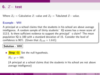
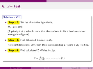


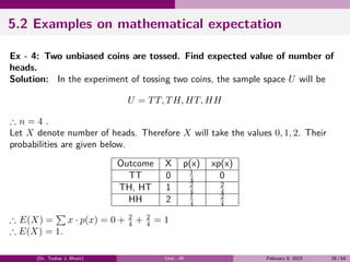
The document provides a comprehensive overview of the theory of probability, including definitions and examples of key concepts such as events, probability, conditional probability, Bayes' theorem, and random variables. It discusses different types of events, the classical definition of probability, and illustrates various examples to demonstrate the application of these principles. Additionally, the document explores the fundamental rules of probability, including the addition and multiplication rules.