Basic probability concept

BASIC PROBABILITY
CONCEPTS
DR MOH MOH KYI

Outlines
■ What is Probability
■ Views of probability
■ Elementary properties of probability
■ Rules of probability
■ Bayes’Theorem

Introduction of probability
■ A good deal of statistical reasoning depends on
probability

Introduction of probability
 Probability theory – foundation for statistical inference
eg. 50-50 chance of surviving an operation
95% certain that he has a stomach cancer
Nine out of ten patients take drugs regularly
 Probability - expressed in terms of percentage (generally) -
 expressed in terms of fractions (mathematically)
 Probability of occurrence – between zero and one

What is probability?
 A number that represents the chance that a particular event will occur
for a random variable.
Eg: Odds of winning a lottery, chance of rolling a seven when rolling two
dice, percent chance of rain in a forecast
 The frequentist definition of probability used in statistics
Betty R. Kirkwood, Jonathan A.C. Sterne, “Essential Medical statistics”, 2nd edition

■ This states that the probability of the occurrence of a particular event equals the
proportion of times that the event would (or does) occur in a large number of similar
repeated trials.

■ Random variable – numerical quantity that takes on different values
depending on chance
■ Population – the set of all possible outcomes for a random variable (
only hypothetical population, not a population of people)
■ An event – an outcome or set of outcomes for a random variable
■ Probability – the proportion of times an event is expected to occur in the
long run. Probabilities are always numbers between 0 and 1
corresponding to always.
B.Burt Gerstman,”Basic Biostatistics,2nd edition

Types of RandomVariables
Discrete random variables
no: of Leukemia cases in geographic region
no: of smokers in a simple random sample of size n
Continuous random variables
Amount of time it take to complete a task
average weight in simple random sample of newborn
the height of individual

Probability of an event
 The probability of an event is viewed as a numerical measure
of the chance that the event will occur.
 Event: An outcome of an experiment or survey.
Eg: rolling a die and turning up six dots
 Elementary event: An outcome that satisfies only one
criterion.
Eg: A red card from a standard deck of cards
 Joint event: An outcome that satisfies two or more criteria
Eg: A red ace from a standard deck of cards

Three basic event operations
 The complement of an event A, denoted by Ā is the set of
all elementary outcomes that are not in A.The occurrence of
Ā means that A does not occur.
 The union of two events A and B, denoted by A U B, is the
set of all elementary outcomes that are in A, B, or both.The
occurrence of A U B means that either A or B or both occur.
Richard A. Johnson, Gouri K. Bhattacharyya, “Statistics: Principles and methods”, 6th edition

Three basic event operations
 The intersection of two events A and B, denoted by A ∩ B,
is the set of all elementary outcomes that are in A and B.The
occurrence of A ∩ B means that both A and B occur.
Note:The operations of union and intersection can be extended
to more than two events.
Richard A. Johnson, Gouri K. Bhattacharyya, “Statistics: Principles and methods”, 6th edition

Two views of Probability
(1) Objective probability
a. Classical or a priori probability
b. Relative frequency or a posteriori probability
(2) Subjective probability

Three views of Probability
Three views of probability:
(1) the subjective-personalistic view,
(2) the classical, or logical view, and
(3) the empirical relative-frequency view
Roger E. Kirk, “Statistics:An introduction”, 5th edition

Objective probability
a. Classical or a priori probability
 A fair six-sided die – Number one --- 1/6
 A well-shuffled playing cards – Heart – 13/52
■ If an event can occur in N mutually exclusive and equally
likely ways, and if m of these possess a trait, E, the
probability of the occurrence of E is equal to m / N.
P (E) = m /N

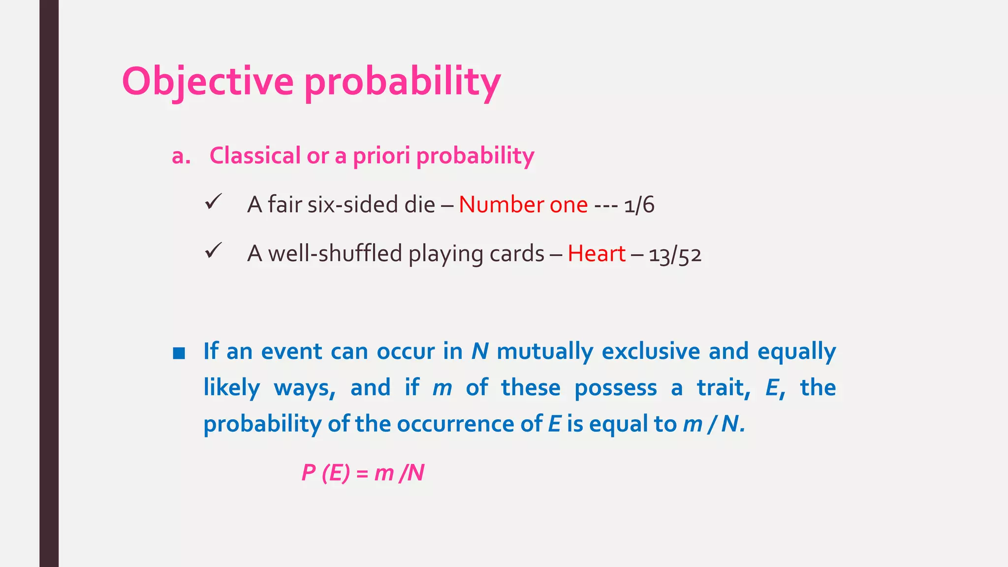
Objective probability
b. Relative frequency or a posteriori probability
 depends on repeatability of some process/ability to count
number of repetitions and number of times that the event
of interest occurs
■ If some process is repeated a large number of times, n,
and if some resulting event with the characteristic E
occurs m times, the relative frequency of occurrence of E,
m /n , will be approximately equal to the probability of E
P (E) = m /n [ m /n is an estimate of P (E) ]

Subjective Probability
 Personalistic or subjective concept of probability
 An event that can occur once eg.The probability that a cure for cancer
will be discovered within the next 10 years.
 Some statisticians do not accept it.

Subjective Probability
 Subjective definition, where the size of the probability simply represents one’s degree
of belief in the occurrence of an event, or in an hypothesis.
 This definition corresponds more closely with everyday usage and is the foundation of
the Bayesian approach to statistics.
 In this approach, the investigator assigns a prior probability to the event (or
hypothesis) under investigation.
 The study is then carried out, the data collected and the probability modified in the
light of the results obtained, using Bayes’ rule.
 The revised probability is called the posterior probability.

Elementary properties of probability
Three properties:
(1) Given some process (or experiment) with n mutually
exclusive outcomes (called events), E1, E2, …., En, the
probability of any event Ei is assigned a nonnegative number.
ie. P(Ei) ≥ 0 (Two mutually exclusive outcomes –Two not
occurring at the same time)
 Mutually exclusive: the probability of both events A and B occurring
is 0.This means that the two events cannot occur at the same time.
Eg: On a single roll of a die, you cannot get a die that has a face
with three dots and also have four dots because such elementary
events are mutually exclusive.

Three properties:
 Mutually exclusive (Incompatible) event
Two events A and B are called incompatible or mutually
exclusive if their intersection AB is empty.

Three properties:
(2)The sum of the probabilities of mutually exclusive outcomes
is equal to 1
P(E1) + P(E2) + … + P(En) = 1
(Property of exhaustiveness –→ all possible events)
 Collectively exhaustive event: A set of events that includes all
the possible events.
Eg: Heads and tails in the toss of a coin, male and female, all
six faces of a die.

Three properties:
(3) Consider any two mutually exclusive events, Ei and Ej.
The probability of the occurrence of either Ei or Ej is equal
to the sum of their individual properties
P(Ei + Ej) = P(Ei) + P(Ej)

Three properties:
1. The probability of an event must be between 0 and 1.The
smallest possible probability value is 0.You cannot have a
negative probability. The largest possible probability value is
1.0.You cannot have a probability greater than 1.0.
2. If events in a set are mutually exclusive and collectively
exhaustive, the sum of their probabilities must add up to 1.0.
3. If two events A and B are mutually exclusive, the probability
of either event A or event B occurring is the sum of their
separate probabilities.
Betty R. Kirkwood, Jonathan A.C. Sterne, “Even you can learn statistics”, 2nd edition

Calculating the probability of an event
Table 1. Frequency of family history of mood disorder by age group
among bipolar subjects
The probability that a person randomly selected from total population
will be 18 year or younger = ?
P (E) = 141 / 318 = 0.4434

Unconditional or Marginal Probability
 One of marginal total was used in numerator and
 The size of total group serve as the denominator
 No conditions were imposed to restrict the size of the
denominator
Conditional Probability
 When probabilities are calculated with a subset of the total
group as the denominator, the result is a conditional
probability

Conditional Probability
 The probability that a person randomly selected from those
18 yr or younger will be the one without family history of
mood disorder=?
 P (A | E) = 28 / 141 = 0.1986
P (A | E) is read as “ probability of A given E”

Joint Probability
 When a person selected possesses two characteristics at
same time, the probability is called ‘joint probability’
 The probability that a person randomly selected from total
population will be early (E) and will be the one without
family history of mood disorder (A) = ?
 P (E ∩ A) = 28 / 318 = 0.0881
(Symbol ∩ is read ‘intersection’ or ‘and’)

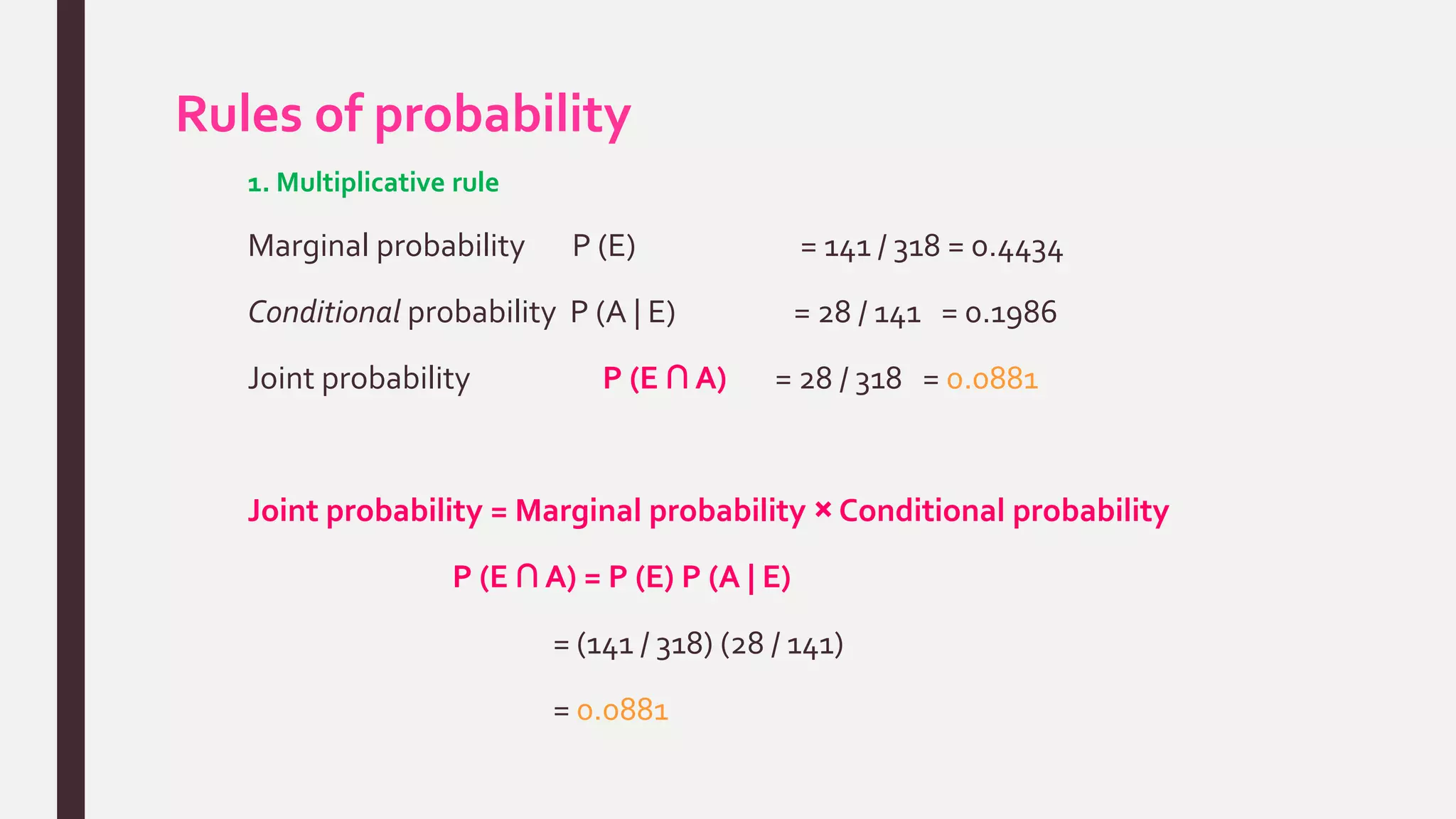
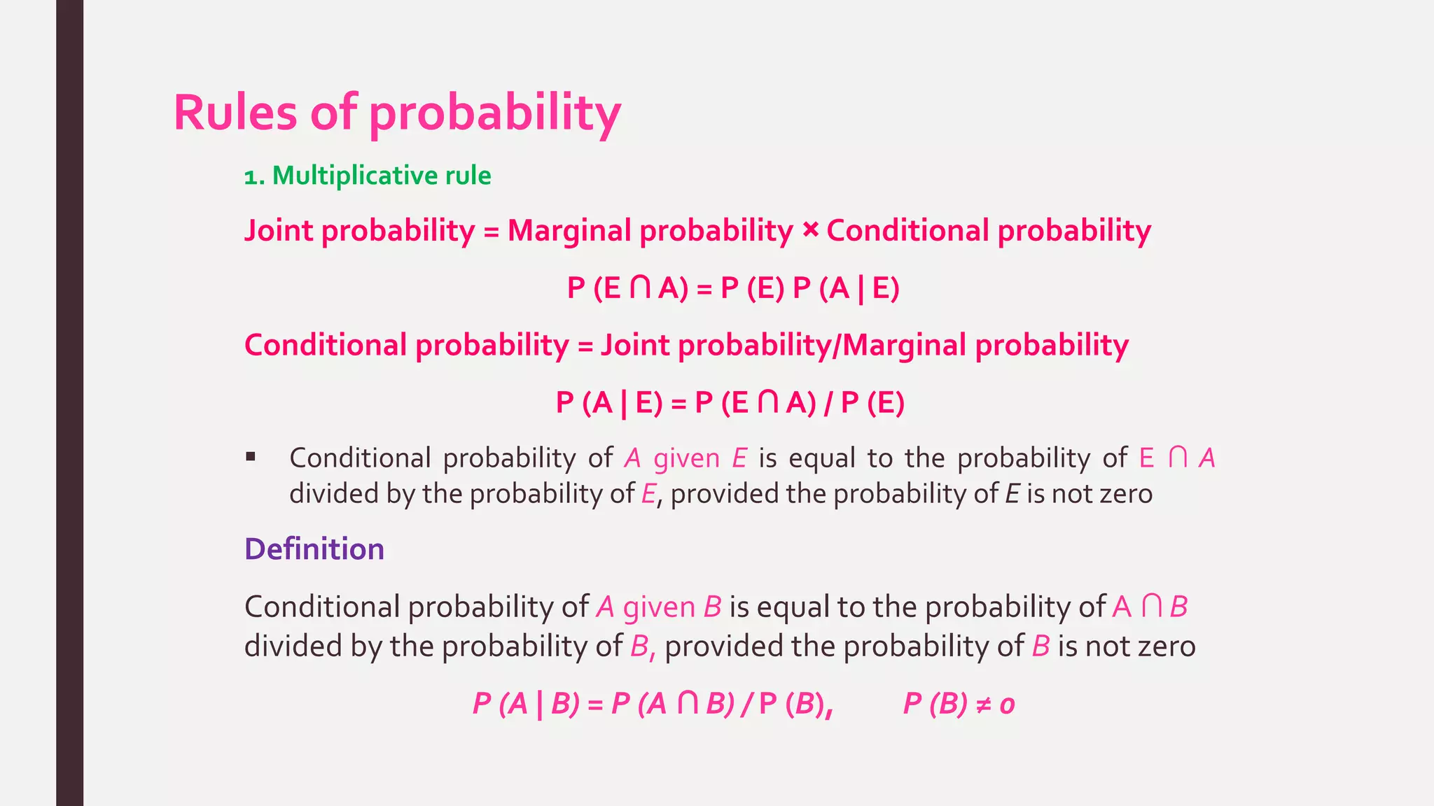
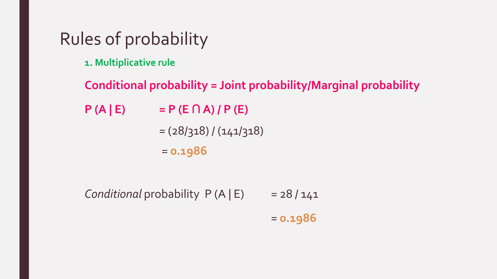
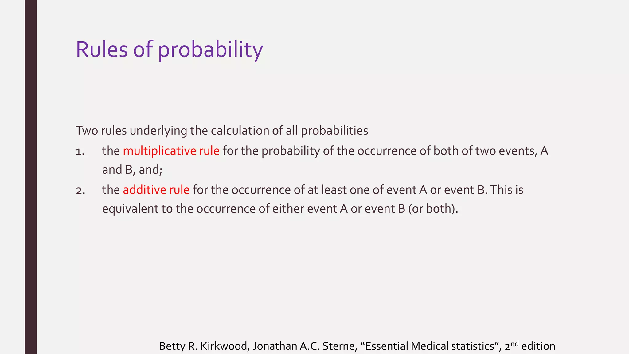
Rules of probability
1. Multiplicative rule
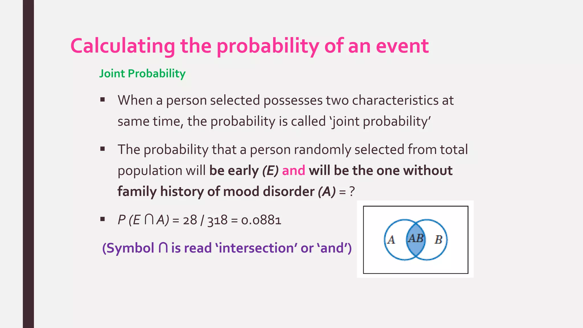
 Joint probability can be calculated as the product of
appropriate marginal probability and appropriate conditional
probability
 This relationship is known as multiplication rule of
probability
P (A ∩ B) = P (B) P (A | B), if P (B) ≠ 0
P (A ∩ B) = P (A) P (B | A), if P (A) ≠ 0
[ Note: P (B), P (A) are marginal probabilities ]

Marginal probability P (E) = 141 / 318 = 0.4434
Conditional probability P (A | E) = 28 / 141 = 0.1986
Joint probability P (E ∩ A) = 28 / 318 = 0.0881
Joint probability = Marginal probability × Conditional probability
P (E ∩ A) = P (E) P (A | E)
= (141 / 318) (28 / 141)
= 0.0881

Joint probability = Marginal probability × Conditional probability
P (E ∩ A) = P (E) P (A | E)
Conditional probability = Joint probability/Marginal probability
P (A | E) = P (E ∩ A) / P (E)
 Conditional probability of A given E is equal to the probability of E ∩ A
divided by the probability of E, provided the probability of E is not zero
Definition
Conditional probability of A given B is equal to the probability of A ∩ B
divided by the probability of B, provided the probability of B is not zero
P (A | B) = P (A ∩ B) / P (B), P (B) ≠ 0

Conditional probability = Joint probability/Marginal probability
P (A | E) = P (E ∩ A) / P (E)
= (28/318) / (141/318)
= 0.1986
Conditional probability P (A | E) = 28 / 141
= 0.1986

2. Additive rule
 The probability of the occurrence of either one or the other of
two mutually exclusive events is equal to the sum of their
individual probabilities (Third property of probability)
 The probability that a person will be early age (E) or later age
(L) = ?
P(E U L) = P (E) + P (L)
= 141/318 + 177/318
= 1
[Symbol ‘U’ is read as ‘union’ or ‘or’]

2. Additive rule
 Given two events A and B, the probability that event A, or event B, or
both occur is equal to the probability that event A occurs, plus the
probability that event B occurs, minus the probability that the events
occur simultaneously (ie not mutually exclusive)
P(A U B) = P (A) + P (B) - P (A ∩ B)
The probability that a person will be an early age (E) or no family h/o (A)
or both = ?
P(E U A) = P (E) + P (A) - P (E ∩ A)
= 141/318 + 63/318 – 28/318
= 0.5534 (duplication/overlapping is adjusted)

Two rules underlying the calculation of all probabilities
1. the multiplicative rule for the probability of the occurrence of both of two events, A
and B, and;
2. the additive rule for the occurrence of at least one of event A or event B.This is
equivalent to the occurrence of either event A or event B (or both).

Independent events
 Occurrence of event B has no effect on the probability of
event A (i.eThe probability of event A is the same regardless
of whether or not B occurs)
i.e. P(A | B) = P(A), P(B | A) = P(B), P(A ∩ B) = P(A) (B)
(if P (A) ≠ 0, P (B) ≠ 0 )
(Note:The terms ‘independent’ and ‘mutually exclusive’ do not mean
the same thing)
 If A an B are independent and event A occurs, the occurrence of B is
not affected.
 If A and B are mutually exclusive, however, and event A occurs,
event B cannot occur.

Example of independent events
Girl (B-) Boy (B) Total
Eyeglasses wearing (E) 24 16 40
No eyeglasses wearing (E-
)
36 24 60
Total 60 40 100
The probability that a person randomly selected wears eyeglasses = ?
P(E) = 40/100 = 0.4
I,eWearing eyeglasses is not concerned
with gender)

Complementary Events
 Given some variable that can be broken down into m categories
designated by A1, A2, …Ai...Am and another jointly occurring
variable that is broken down to n categories designated by B1,
B2…Bj...Bn, the marginal probability of Ai, P(Ai) , is equal to the sum
of the joint probabilities of Ai with all the categories of B.
P(Ai) = ΣP(Ai ∩ Bj ), for all value of j
Example: P (B) = 1- P (B-)
B and B- are complementary events
Event B and its complement event B- are mutually exclusive
(third property of probability)

BAYES’THEOREM
 Thomas Bayes, an English Clergyman (1702-1761)
 Estimates of the predictive value positive and predictive
value negative of a test → based on test’s sensitivity,
specificity and probability of the relevant disease in general
population
 Bayes’ rule for relating conditional probabilities:

BAYES’THEOREM
Suppose that we know that 10% of young girls in India are malnourished,
and that 5% are anaemic, and that we are interested in the relationship
between the two. Suppose that we also know that 50% of anaemic girls are
also alnourished. This means that the two conditions are not independent,
since if they were then only 10% (not 50%) of anaemic girls would also be
malnourished, the same proportion as the population as a whole. However,
we don’t know the relationship the other way round, that is what
percentage of malnourished girls are also anaemic. We can use Bayes’ rule
to deduce this.

BAYES’THEOREM
Probability (malnourished) = 0.1
Probability (anaemic) = 0.05
Probability (malnourished given anaemic) = 0.5
Using Bayes rule gives:
Prob (anaemic given malnourished)
We can thus conclude that 25%, or one quarter, of malnourished girls
are also anaemic.

Sensitivity
The sensitivity of a test (or symptom) is the probability of a positive test result (or
presence of the symptom) given the presence of the disease.

Specificity
The specificity of a test (or symptom) is the probability of a negative test result (or
absence of the symptom) given the absence of the disease.

Predictive value positive
The predictive value positive of a screening test (or symptom) is the probability that
a subject has the disease given that the subject has a positive screening test result (or
has the symptom)

Predictive value negative
The predictive value negative of a screening test (or symptom) is the probability that
a subject does not have the disease given that the subject has a negative screening
test result (or does not have the symptom)

BAYES’THEOREM
 Predictive value positive of a screening test (or symptom)
 Predictive value negative of a screening test (or symptom)

Example
Sensitivity of the test
P(T/D) = 436 / 450 = 0.9689
Specificity of the test
P(T-/D-) = 495 / 500 = 0.99

Example
Sensitivity of the test
P(T/D) = 436 / 450 = 0.9689
Specificity of the test
P(T-/D-) = 495 / 500 = 0.99
Predictive value positive of the test
If P(D) = 0.113 (11.3% of the U.S population aged 65 and over have
Alzheimer’s disease)

Example
Predictive value positive of the test
If P(D) = 0.113 (11.3% of the U.S population aged 65 and over haveAlzheimer’s
disease)
Predictive value of positive test is very high.
*The predictive value positive of the test depends on the rate of the disease
in the relevant population in general

Example
Predictive value negative of the test
The predictive value negative is also quite high.

Normal Distribution
 Also known as Gaussian distribution [Carl Friedrich Gauss (1777-1855)]
Normal density

Characteristics of Normal Distribution
1. It is symmetrical about the mean, µ .The curve on either side
of µ is mirror image of the other side
2.The mean, the median and mode are all equal.

3. The total area under the curve above the x axis is one square
unit. Normal distribution is probability distribution. 50% of
the area is to the right of a perpendicular erected at the
mean and 50% is to the left.

4. 1 SD from the mean in both directions, the area is 68%.
For 2 SD and 3 SD, areas are 95% and 99.7% respectively

5.The normal distribution is determined by µ and σ
Different values of µ cause the distribution graph shift along
the x axis
Therefore, µ is often referred to as a location parameter

5.The normal distribution is determined by µ and σ
Different values of σ cause the degree of flatness or
peakedness of distribution graphs
σ is often referred to as a shape parameter

Homework
Page 76 3.4.1, 3.4.5, 3.4.6
Page 83 3.5.1
Page 85 3,6,13

Basic probability concept

Recommended

Recommended

More Related Content

What's hot

What's hot (20)

Similar to Basic probability concept

Similar to Basic probability concept (20)

More from Mmedsc Hahm

More from Mmedsc Hahm (20)

Recently uploaded

Recently uploaded (20)

Basic probability concept