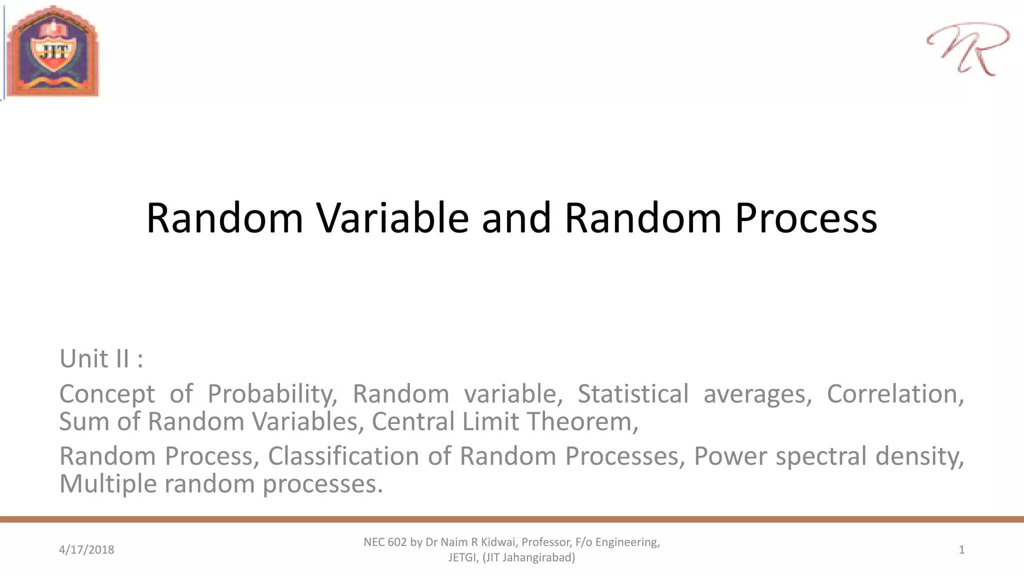
Nec 602 unit ii Random Variables and Random process

Random Variable and Random Process
Unit II :
Concept of Probability, Random variable, Statistical averages, Correlation,
Sum of Random Variables, Central Limit Theorem,
Random Process, Classification of Random Processes, Power spectral density,
Multiple random processes.
4/17/2018 1
NEC 602 by Dr Naim R Kidwai, Professor, F/o Engineering,
JETGI, (JIT Jahangirabad)

Concept of Probability
4/17/2018 2
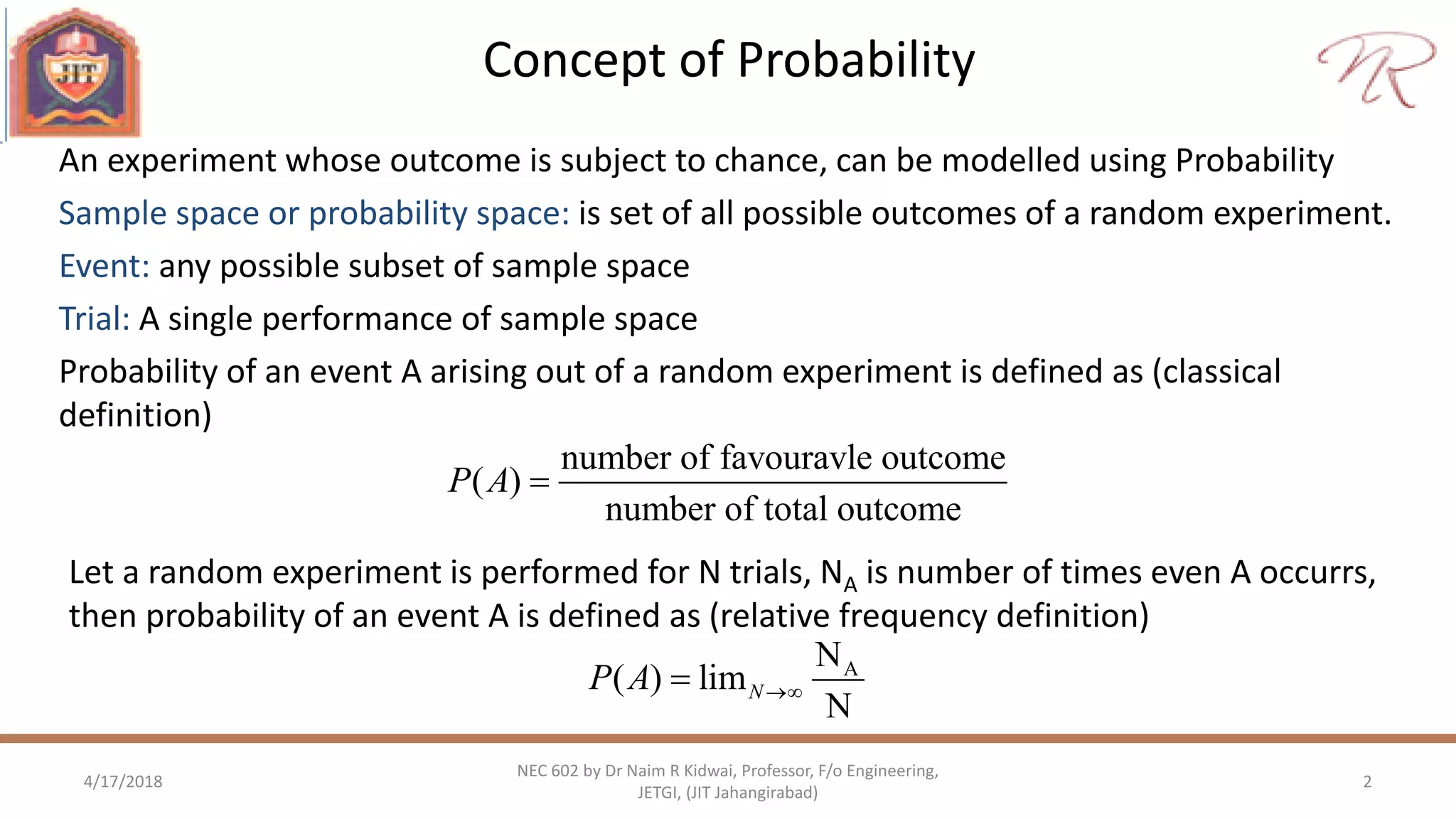
An experiment whose outcome is subject to chance, can be modelled using Probability
Sample space or probability space: is set of all possible outcomes of a random experiment.
Event: any possible subset of sample space
Trial: A single performance of sample space
Probability of an event A arising out of a random experiment is defined as (classical
definition)
number of favouravle outcome
( )
number of total outcome
P A 
Let a random experiment is performed for N trials, NA is number of times even A occurrs,
then probability of an event A is defined as (relative frequency definition)
AN
( ) lim
N
NP A 

4/17/2018 3
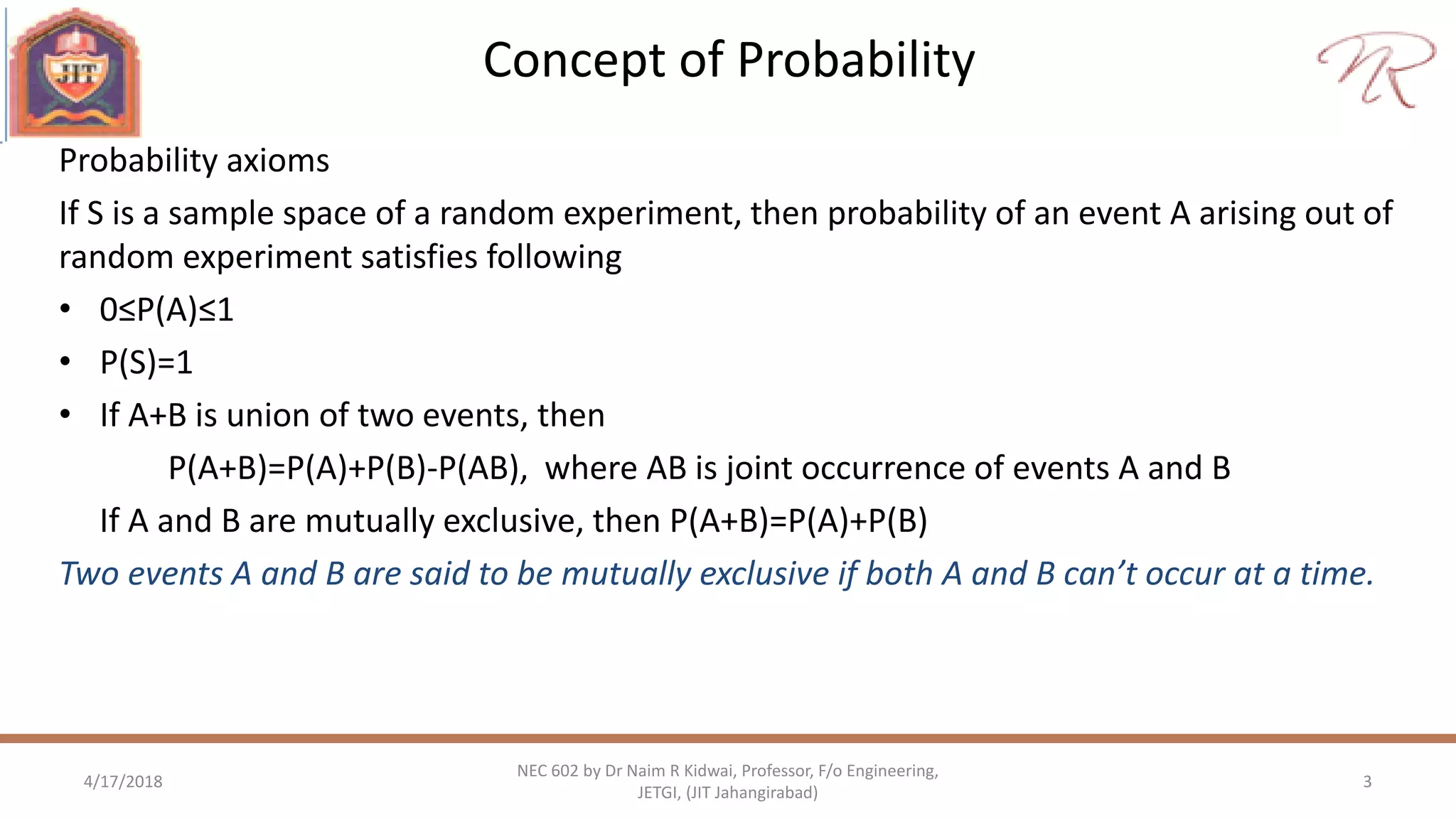
Probability axioms
If S is a sample space of a random experiment, then probability of an event A arising out of
random experiment satisfies following
• 0≤P(A)≤1
• P(S)=1
• If A+B is union of two events, then
P(A+B)=P(A)+P(B)-P(AB), where AB is joint occurrence of events A and B
If A and B are mutually exclusive, then P(A+B)=P(A)+P(B)
Two events A and B are said to be mutually exclusive if both A and B can’t occur at a time.

4/17/2018 4
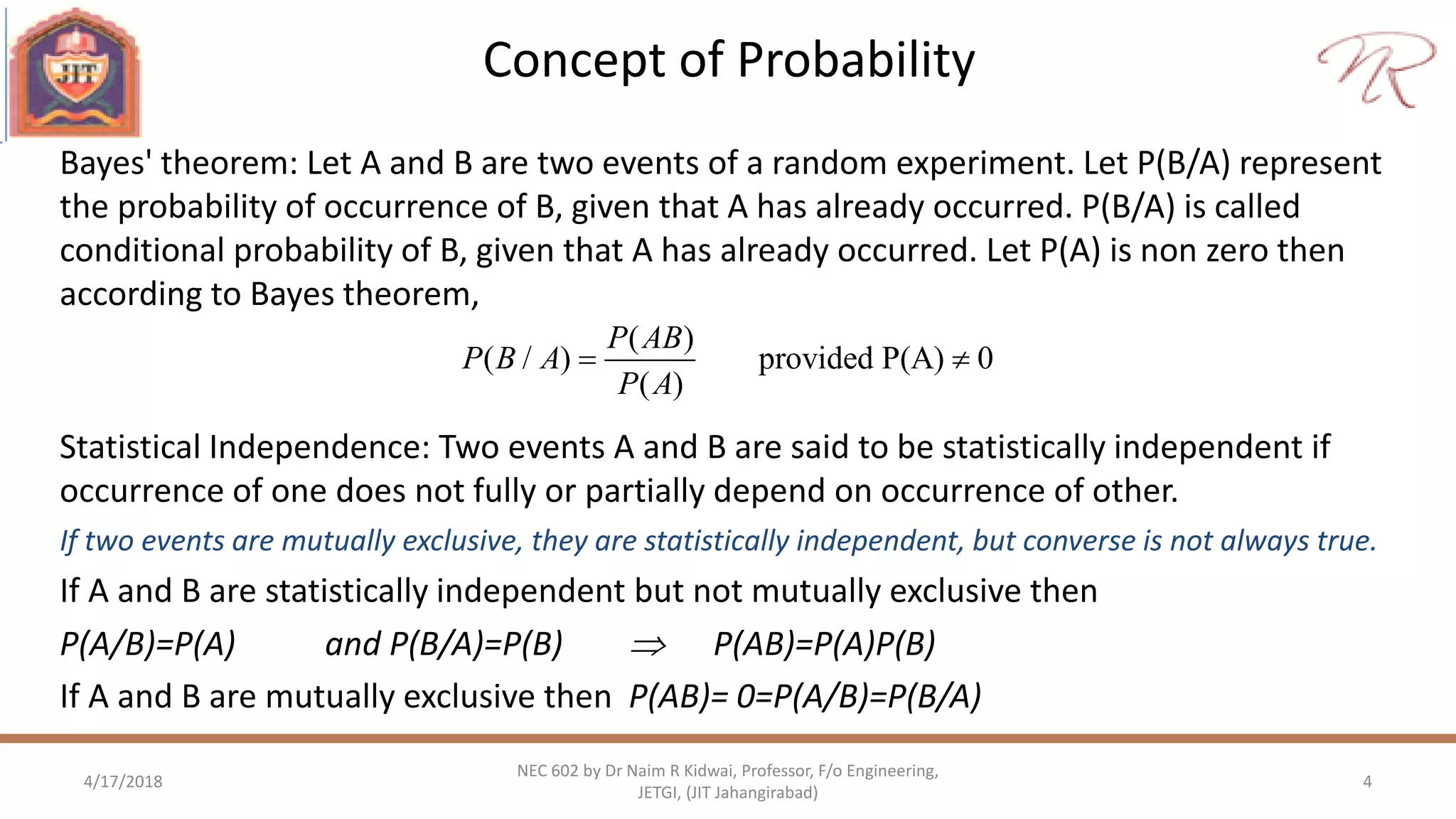
Bayes' theorem: Let A and B are two events of a random experiment. Let P(B/A) represent
the probability of occurrence of B, given that A has already occurred. P(B/A) is called
conditional probability of B, given that A has already occurred. Let P(A) is non zero then
according to Bayes theorem,
( )
( / ) provided P(A) 0
( )
P AB
P B A
P A
 
Statistical Independence: Two events A and B are said to be statistically independent if
occurrence of one does not fully or partially depend on occurrence of other.
If two events are mutually exclusive, they are statistically independent, but converse is not always true.
If A and B are statistically independent but not mutually exclusive then
P(A/B)=P(A) and P(B/A)=P(B)  P(AB)=P(A)P(B)
If A and B are mutually exclusive then P(AB)= 0=P(A/B)=P(B/A)

4/17/2018 5
Bayes' theorem: Let A and B are two events of a random experiment. Let P(B/A) represent
the probability of occurrence of B, given that A has already occurred. P(B/A) is called
conditional probability of B, given that A has already occurred. Let P(A) is non zero then
according to Bayes theorem,
( )
( / ) provided P(A) 0
( )
P AB
P B A
P A
 
Statistical Independence: Two events A and B are said to be statistically independent if
occurrence of one does not fully or partially depend on occurrence of other.
If two events are mutually exclusive, they are statistically independent, but converse is not always true.
If A and B are statistically independent but not mutually exclusive then
P(A/B)=P(A) and P(B/A)=P(B)  P(AB)=P(A)P(B)
If A and B are mutually exclusive then P(AB)= 0=P(A/B)=P(B/A)

Random variable
4/17/2018 6
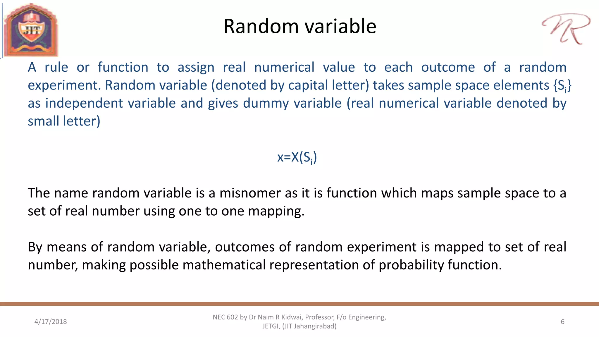
A rule or function to assign real numerical value to each outcome of a random
experiment. Random variable (denoted by capital letter) takes sample space elements {Si}
as independent variable and gives dummy variable (real numerical variable denoted by
small letter)
x=X(Si)
The name random variable is a misnomer as it is function which maps sample space to a
set of real number using one to one mapping.
By means of random variable, outcomes of random experiment is mapped to set of real
number, making possible mathematical representation of probability function.

Discrete Random variable
4/17/2018 7
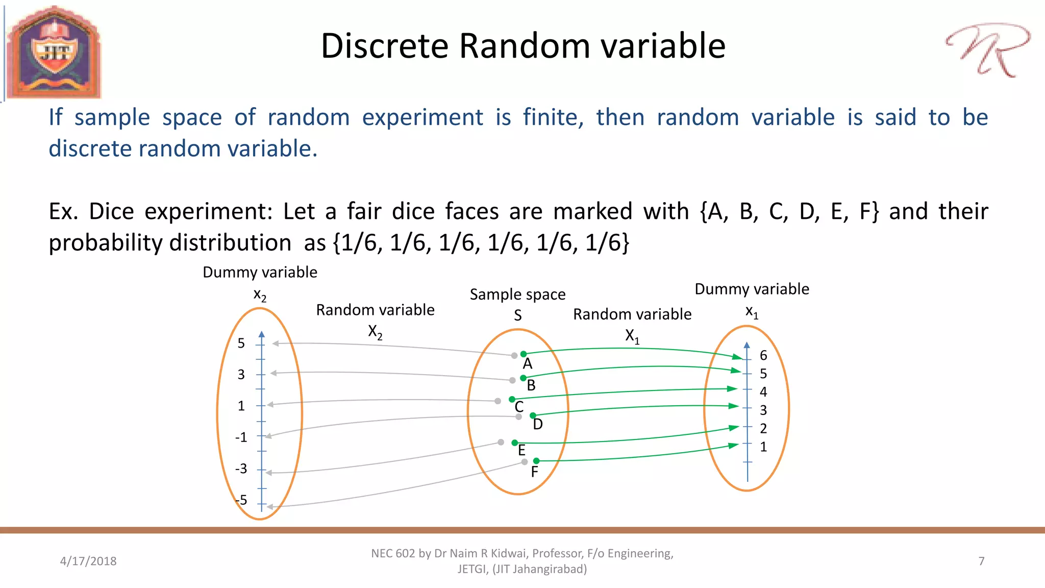
If sample space of random experiment is finite, then random variable is said to be
discrete random variable.
Ex. Dice experiment: Let a fair dice faces are marked with {A, B, C, D, E, F} and their
probability distribution as {1/6, 1/6, 1/6, 1/6, 1/6, 1/6}
Random variable
X2
A
C
B
E
D
F
6
5
4
3
2
1
Sample space
S
Dummy variable
x1
5
3
1
-1
-3
-5
Dummy variable
x2
Random variable
X1

Continuous random variable Random variable
4/17/2018 8
If sample space of random experiment is infinite, then random variable is said to be
continuous random variable.
Ex. Pointer spinning experiment: Let a pointer P attached to origin on a horizontal table can
move in a circle. After movement pointer stops at a point which makes an angle with x-axis.
For continuous random variable, probability is defined in a range and not on a point.
Probability of a point in continuous random variable is zero.
For pointer spinning experiment P(<x≤+d) = P(<X≤+d)
P
O

Random variable X2
Sample space S Dummy variable x1
+0 +2
Dummy variable x2
Random variable X1

0 2

- 


Cumulative Distribution Function (cdf)
4/17/2018 9
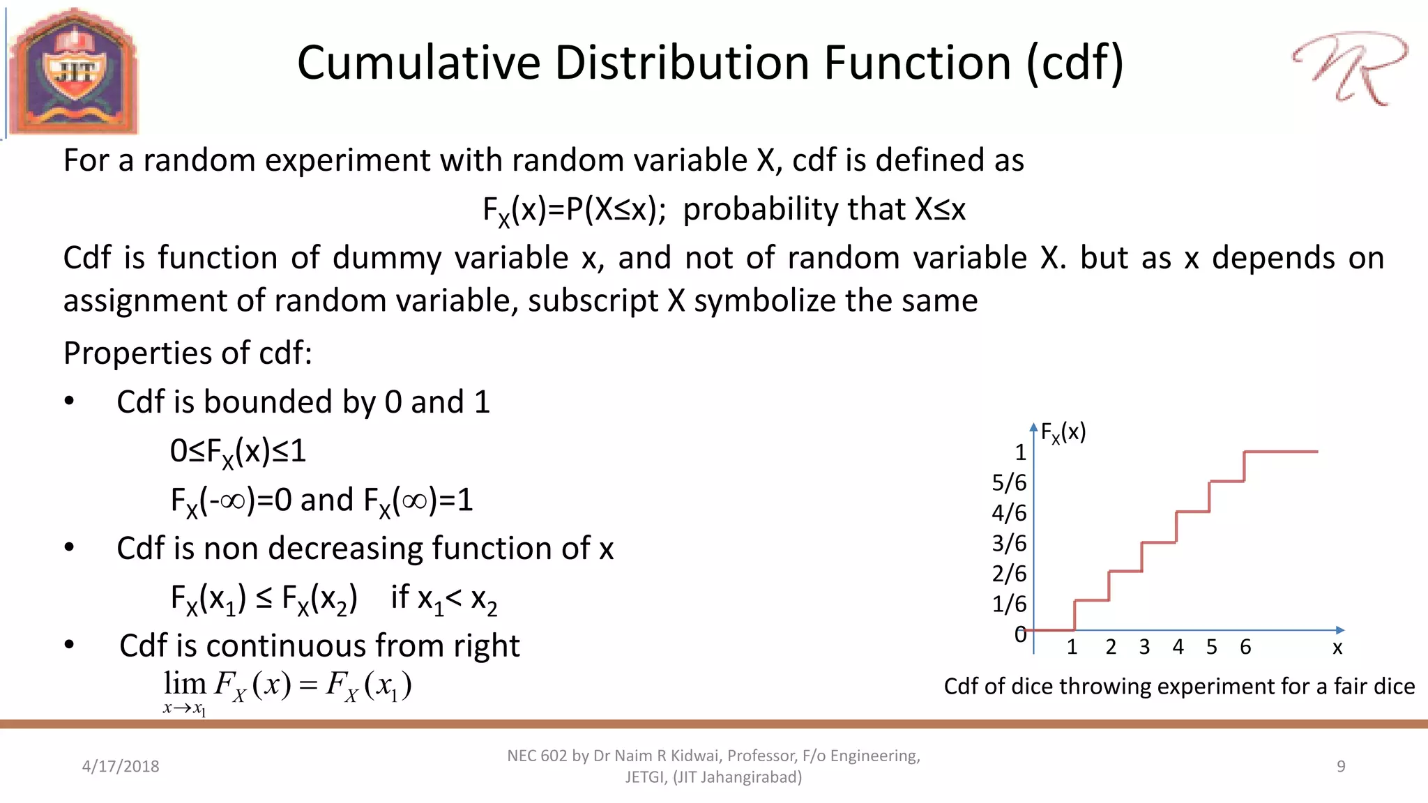
For a random experiment with random variable X, cdf is defined as
FX(x)=P(X≤x); probability that X≤x
Cdf is function of dummy variable x, and not of random variable X. but as x depends on
assignment of random variable, subscript X symbolize the same
1
5/6
4/6
3/6
2/6
1/6
0 1 2 3 4 5 6 x
FX(x)
Cdf of dice throwing experiment for a fair dice
Properties of cdf:
• Cdf is bounded by 0 and 1
0≤FX(x)≤1
FX(-)=0 and FX()=1
• Cdf is non decreasing function of x
FX(x1) ≤ FX(x2) if x1< x2
• Cdf is continuous from right
1
1lim ( ) ( )X X
x x
F x F x



Probability Density Function (pdf)
4/17/2018 10
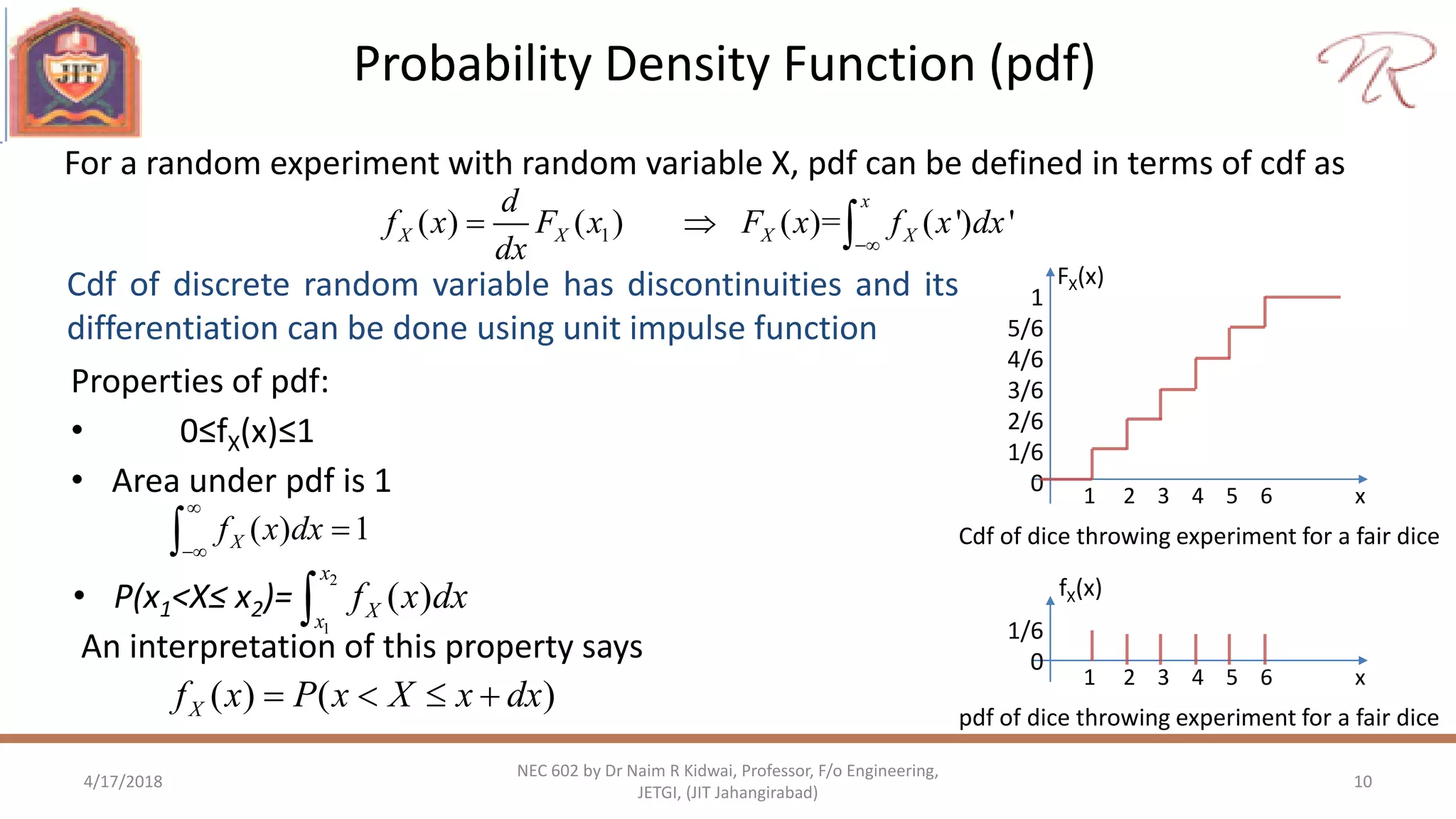
For a random experiment with random variable X, pdf can be defined in terms of cdf as
1
5/6
4/6
3/6
2/6
1/6
0 1 2 3 4 5 6 x
FX(x)
Cdf of dice throwing experiment for a fair dice
Properties of pdf:
• 0≤fX(x)≤1
• Area under pdf is 1
1( ) ( ) ( )= ( ') '
x
X X X X
d
f x F x F x f x dx
dx 
  
Cdf of discrete random variable has discontinuities and its
differentiation can be done using unit impulse function
( ) 1Xf x dx



• P(x1<X≤ x2)=
An interpretation of this property says
2
1
( )
x
Xx
f x dx
( ) ( )Xf x P x X x dx   
1/6
0
1 2 3 4 5 6 x
fX(x)
pdf of dice throwing experiment for a fair dice

Cdf, Pdf example: double dice throwing experiment
4/17/2018 11
Two fair dices are thrown in an experiment. Let
sum of faces of two dices is random variable X.
X Possible outcomes of the dice P(X=x) Cumulative
probability P(X≤x)
2 (1,1) 1/36 1/36
3 (1,2), (2,1) 2/36 3/36
4 (1,3), (2,2), (3,1) 3/36 6/36
5 (1,4), (2,3), (3,2), (4,1) 4/36 10/36
6 (1,5), (2,4), (3,3), (4,2), (5,1) 5/56 15/36
7 (1,6), (2,5), (3,4), (4,3), (5,2), (6,1) 6/36 21/36
8 (2,6), (3,5), (4,4), (5,3), (6,2) 5/36 26/36
9 (3,6), (4,5), (5,4), (6,3) 4/36 30/36
10 (4,6), (5,5), (6,4) 3/36 33/36
11 (5,6), (6,5) 2/36 35/36
12 (6,6) 1/36 1
cdf of double dice throwing experiment
1
30/36
24/36
18/36
12/36
6/36
0
2 3 4 5 6 7 8 9 10 11 12 x
FX(x)
pdf of double dice throwing experiment
6/36
5/36
4/36
3/36
2/36
1/36
0 2 3 4 5 6 7 8 9 10 11 12 x
fX(x)

Joint pdf /cdf, marginal pdf/cdf
4/17/2018 12
Joint pdf/cdf
A random experiment may be characterized
by using two or more random variables.
Pdf/cdf of such experiment is referred as
joint pdf or joint cdf.
,
2
, ,
, ,
joint cdf ( , ) ( and )
joint pdf ( , ) ( , )
and ( , ) ( ', ') ' '
X Y
X Y X Y
yx
X Y X Y
F x y P X x Y y
f x y F x y
x y
F x y f x y dx dy
 
  


 
  
Marginal pdf/cdf
Pdf/cdf of a single random variable can
be obtained from joint pdf /cdf, referred
as marginal pdf/cdf
,
,
,
marginal cdf ( ) ( , )
marginal pdf ( ) ( , )
( , ') '
X X Y
X X Y
X Y
F x F x
d
f x F x y
dx
f x y dy


 

 

Joint pdf /cdf, example
4/17/2018 13
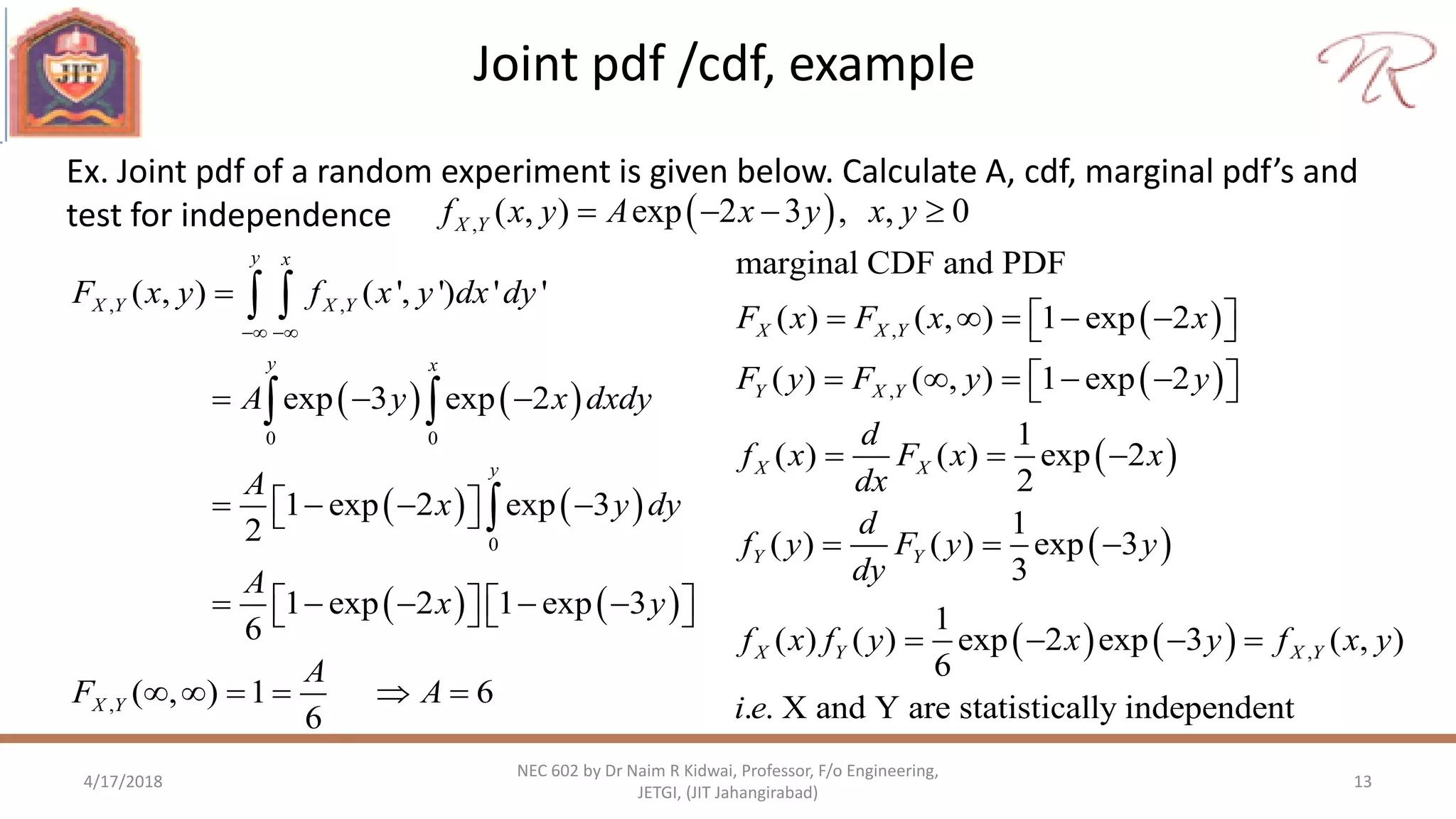
Ex. Joint pdf of a random experiment is given below. Calculate A, cdf, marginal pdf’s and
test for independence  , ( , ) exp 2 3 , , 0X Yf x y A x y x y   
   
   
   
, ,
0 0
0
,
( , ) ( ', ') ' '
exp 3 exp 2
1 exp 2 exp 3
2
1 exp 2 1 exp 3
6
( , ) 1 6
6
y x
X Y X Y
y x
y
X Y
F x y f x y dx dy
A y x dxdy
A
x y dy
A
x y
A
F A
 

  
     
          
     
 
 

 
 
 
 
   
,
,
,
marginal CDF and PDF
( ) ( , ) 1 exp 2
( ) ( , ) 1 exp 2
1
( ) ( ) exp 2
2
1
( ) ( ) exp 3
3
1
( ) ( ) exp 2 exp 3 ( , )
6
. . X and Y are statistically independent
X X Y
Y X Y
X X
Y Y
X Y X Y
F x F x x
F y F y y
d
f x F x x
dx
d
f y F y y
dy
f x f y x y f x y
i e
      
      
  
  
   

Transformation of random variable
4/17/2018 14
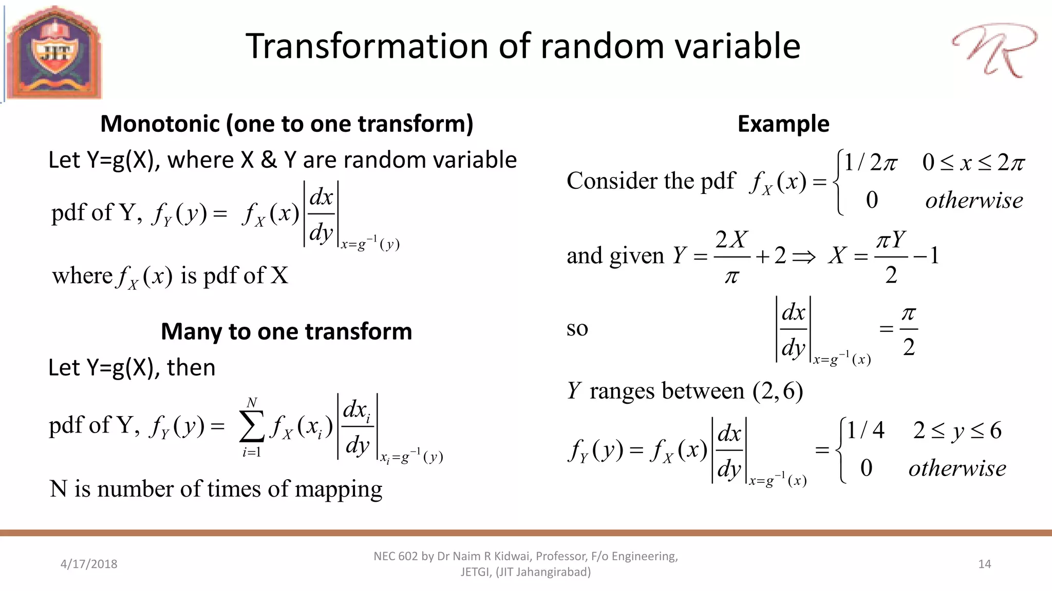
Monotonic (one to one transform)
Let Y=g(X), where X & Y are random variable
Example
1
( )
pdf of Y, ( ) ( )
where ( ) is pdf of X
Y X
x g y
X
dx
f y f x
dy
f x



Many to one transform
Let Y=g(X), then
11 ( )
pdf of Y, ( ) ( )
N is number of times of mapping
i
N
i
Y X i
i x g y
dx
f y f x
dy  
 
1
1
( )
( )
1/ 2 0 2
Consider the pdf ( )
0
2
and given 2 1
2
so
2
ranges between (2,6)
1/ 4 2 6
( ) ( )
0
X
x g x
Y X
x g x
x
f x
otherwise
X Y
Y X
dx
dy
Y
ydx
f y f x
otherwisedy
 







 
 

    

 
  


Statistical Averages: mean
4/17/2018 15
Pdf and cdf provide probabilistic characterization of random variable. Partial
description of random variable are given in form of statistical averages.
[ ] ( )
Let ( ), where X, Y random variables
then [ ] ( ) ( )
X X
Y X
E X xf x dx
Y g X
E Y g x f x dx






 
 
 


Average or Mean or Expectation:

Statistical Averages: Moment and central moment
4/17/2018 16
nth central moment
th
st
nd 2
n moment of random variable
[ ] ( )
1 moment [ ] mean
2 moment [ ] mean square
n n
XE X x f x dx
E X
E X






nth moment
th
st
nd 2 2 2 2
2
n central moment of random variable
[( ) ] ( ) ( )
1 central moment [( )] 0
2 moment [( ) ] [ ]
Variance of X,
standard deviation of X
n n
X X X
X
X X X
X
X
E X x f x dx
E X
E X E X
 

  




  
 
   




Statistical Averages: Joint Moments
4/17/2018 17
,order i+j moment, [ ] ( , )
If X and Y are statistically independent then [ ] [ ] [ ]
i j i j
X Y
i j i j
E X Y x y f x y dxdy
E X Y E X E Y
 
 


 
Order i+j moment : Let X and Y are random variables with joint pdf fX,Y(x,y)
Correlation: E[XY] is referred as correlation
Covariance: COV[XY]=E[(X-X) (Y-Y)] = E[XY] - X Y is referred as covariance of X and Y
[ ]
Correlation coefficient,
1 1
0 no correlation,
1 Y and X are linearly dependent
XY
X Y
XY
XY
XY
Cov XY

 




  
 
  

Sum of Random Variables
4/17/2018 18
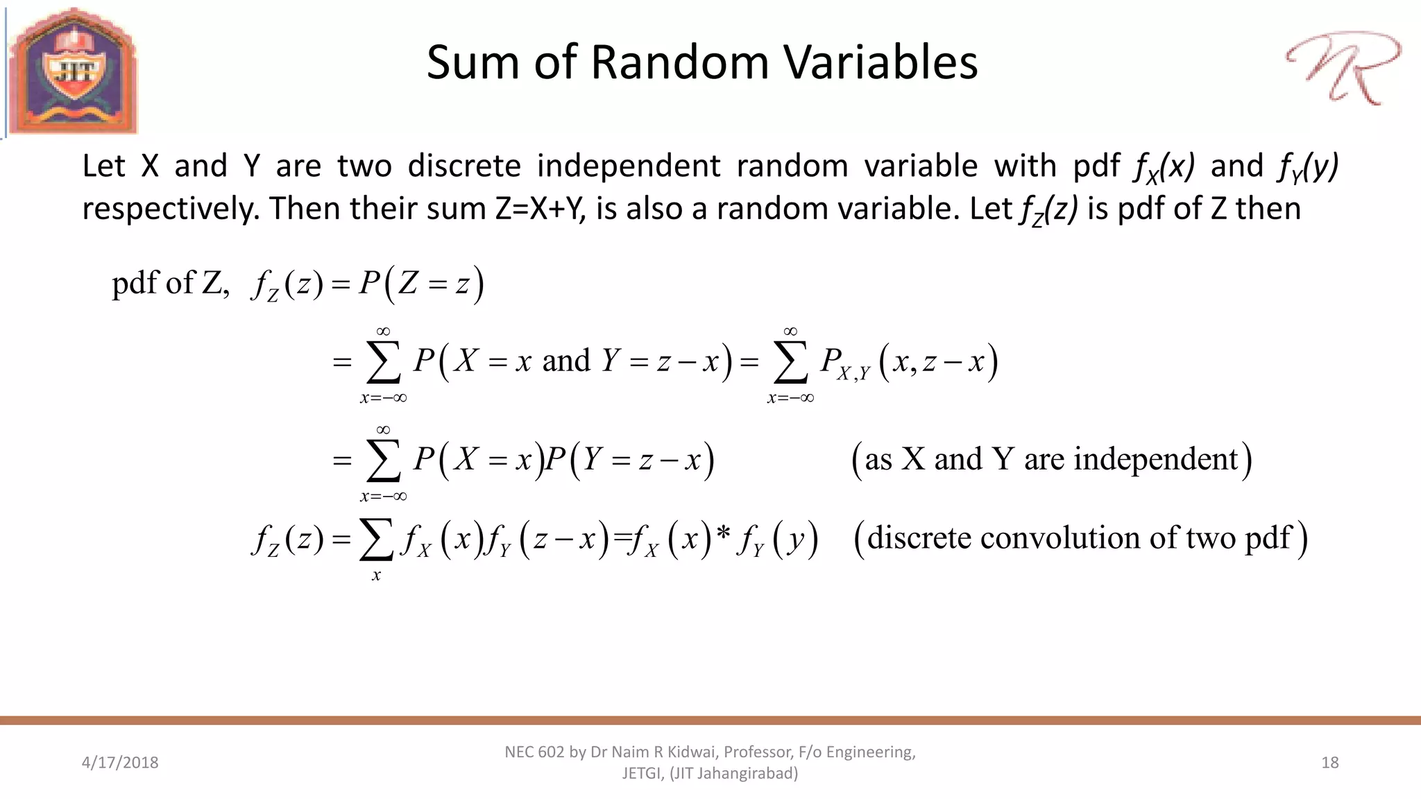
Let X and Y are two discrete independent random variable with pdf fX(x) and fY(y)
respectively. Then their sum Z=X+Y, is also a random variable. Let fZ(z) is pdf of Z then
 
   
     
   
,
pdf of Z, ( )
and ,
as X and Y are independent
( )
Z
X Y
x x
x
Z X Y
x
f z P Z z
P X x Y z x P x z x
P X x P Y z x
f z f x f z x
 
 


 
     
   
 
 

      = * discrete convolution of two pdfX Yf x f y

Central Limit Theorem (CLT)
4/17/2018 19
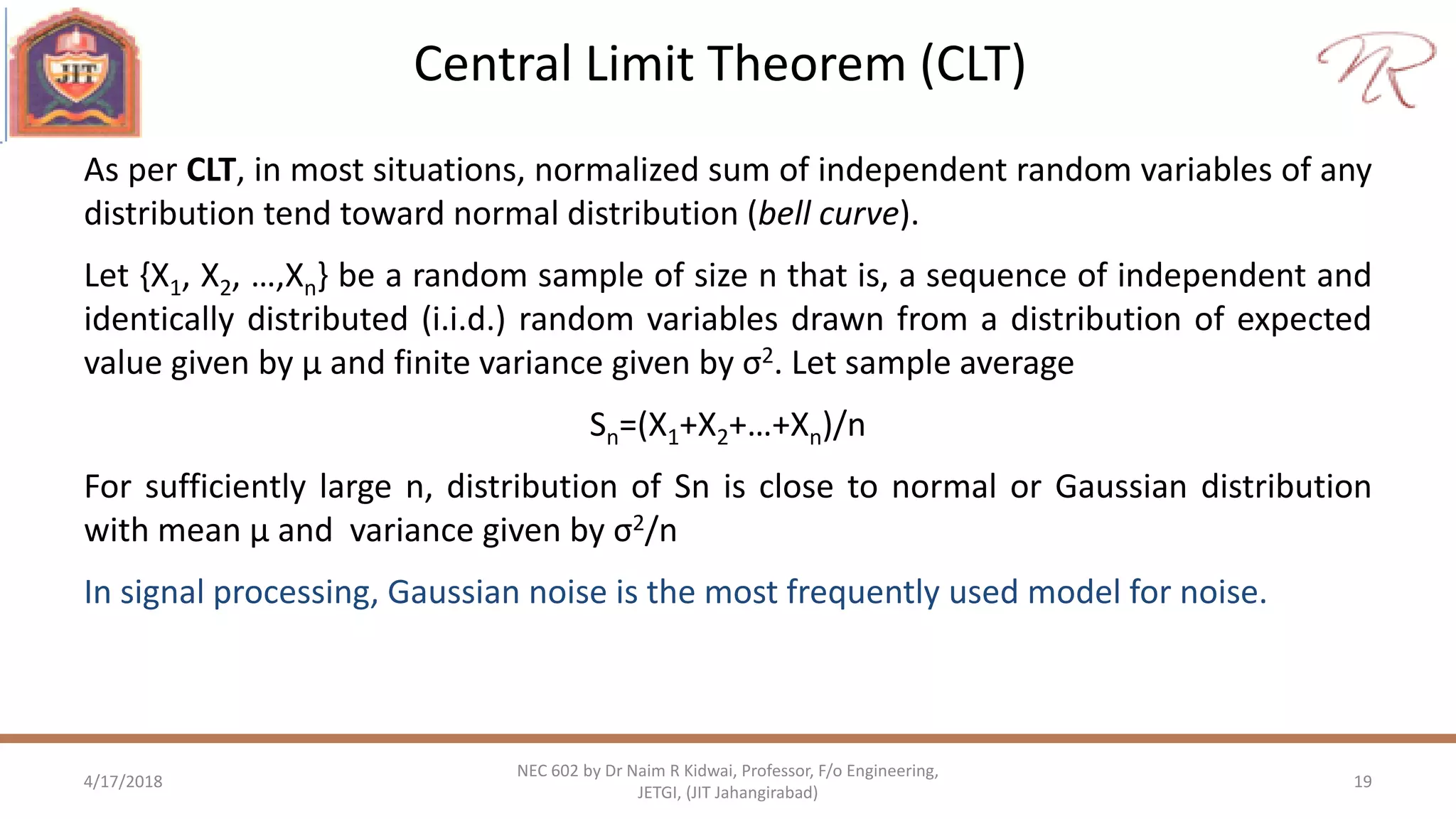
As per CLT, in most situations, normalized sum of independent random variables of any
distribution tend toward normal distribution (bell curve).
Let {X1, X2, …,Xn} be a random sample of size n that is, a sequence of independent and
identically distributed (i.i.d.) random variables drawn from a distribution of expected
value given by µ and finite variance given by σ2. Let sample average
Sn=(X1+X2+…+Xn)/n
For sufficiently large n, distribution of Sn is close to normal or Gaussian distribution
with mean µ and variance given by σ2/n
In signal processing, Gaussian noise is the most frequently used model for noise.

Random Process or Stochastic Process (Random Signals)
4/17/2018 20
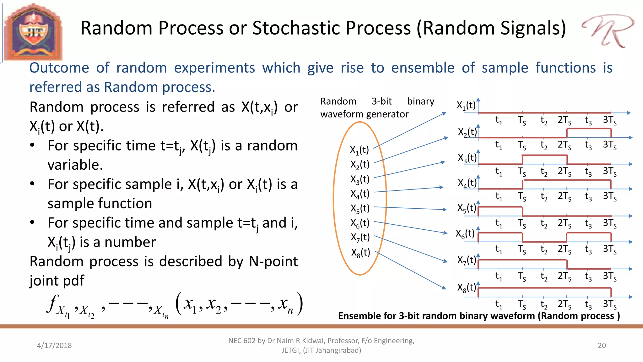
Random process is referred as X(t,xi) or
Xi(t) or X(t).
• For specific time t=tj, X(tj) is a random
variable.
• For specific sample i, X(t,xi) or Xi(t) is a
sample function
• For specific time and sample t=tj and i,
Xi(tj) is a number
Random process is described by N-point
joint pdf
TS 2TS 3TSt1 t2 t3
TS 2TS 3TSt1 t2 t3
TS 2TS 3TSt1 t2 t3
TS 2TS 3TSt1 t2 t3
TS 2TS 3TSt1 t2 t3
TS 2TS 3TSt1 t2 t3
TS 2TS 3TSt1 t2 t3
TS 2TS 3TSt1 t2 t3
X1(t)
X2(t)
X3(t)
X4(t)
X5(t)
X6(t)
X7(t)
X8(t)
X1(t)
X2(t)
X3(t)
X4(t)
X5(t)
X6(t)
X7(t)
X8(t)
Random 3-bit binary
waveform generator
Ensemble for 3-bit random binary waveform (Random process )
Outcome of random experiments which give rise to ensemble of sample functions is
referred as Random process.
 1 2
1 2, , , , , ,t t tn
X X X nf x x x     

Random Process : Important moments
4/17/2018 21
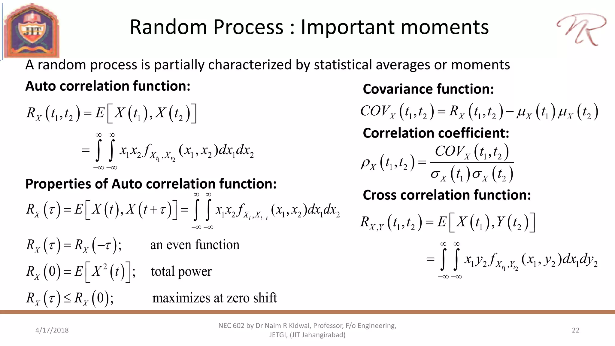
A random process is partially characterized by statistical averages or moments
1
( ) 1 1 1[ ( )] ( )tX t XE X t x f x dx


  
Mean or Expectation of X(t):
Variance of X(t)
      
    1
22
2
1 1 1t
X X
X X
t E X t t
x t f x dx
 



  
 
 
• Mean of random process is generally function of time
• Variance & standard deviation of random process is generally function of time

Random Process : Important moments
4/17/2018 22
A random process is partially characterized by statistical averages or moments
     
1 2
1 2 1 2
1 2 , 1 2 1 2
, ,
( , )t t
X
X X
R t t E X t X t
x x f x x dx dx
 
 
   
  
Auto correlation function:
       1 2 1 2 1 2, ,X X X XCOV t t R t t t t  
Covariance function:
 
 
   
1 2
1 2
1 2
,
, X
X
X X
COV t t
t t
t t

 

Correlation coefficient:
     
1 2
, 1 2 1 2
1 2 , 1 2 1 2
, ,
( , )t t
X Y
X Y
R t t E X t Y t
x y f x y dx dy
 
 
   
  
Cross correlation function:
Properties of Auto correlation function:
     
   
   
   
1 2 , 1 2 1 2
2
, ( , )
; an even function
0 ; total power
0 ; maximizes at zero shift
t tX X X
X X
X
X X
R E X t X t x x f x x dx dx
R R
R E X t
R R

 
 


 
 
    
 
   

 

Classification of Random Processes
4/17/2018 23
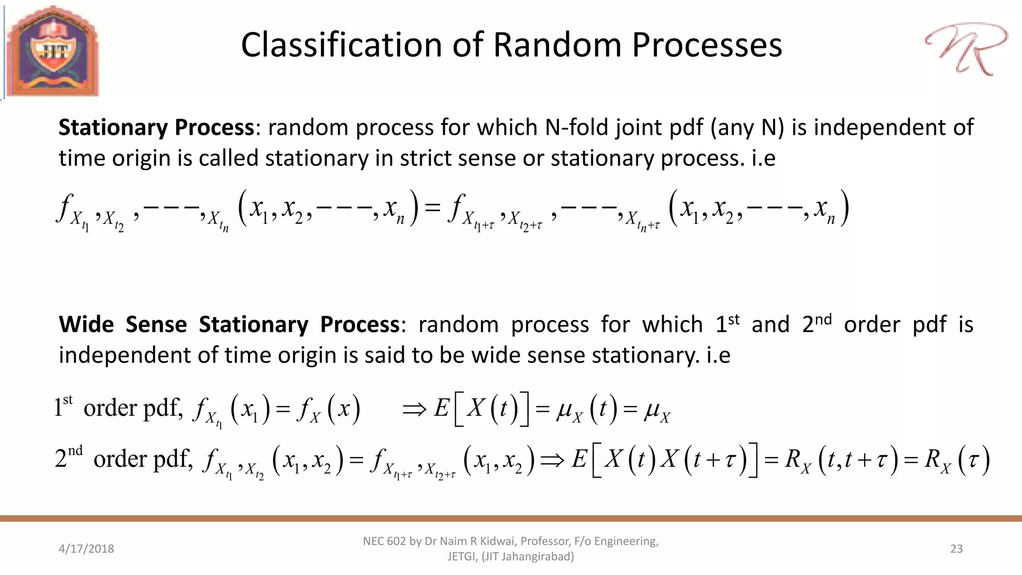
Stationary Process: random process for which N-fold joint pdf (any N) is independent of
time origin is called stationary in strict sense or stationary process. i.e
Wide Sense Stationary Process: random process for which 1st and 2nd order pdf is
independent of time origin is said to be wide sense stationary. i.e
   1 2 1 2
1 2 1 2, , , , , , , , , , , ,t t t t t tn n
X X X n X X X nf x x x f x x x    
            
       
           
1
1 2 1 2
st
1
nd
1 2 1 2
1 order pdf,
2 order pdf, , , , , ,
t
t t t t
X X X X
X X X X X X
f x f x E X t t
f x x f x x E X t X t R t t R 
 
   
     
       

4/17/2018 24
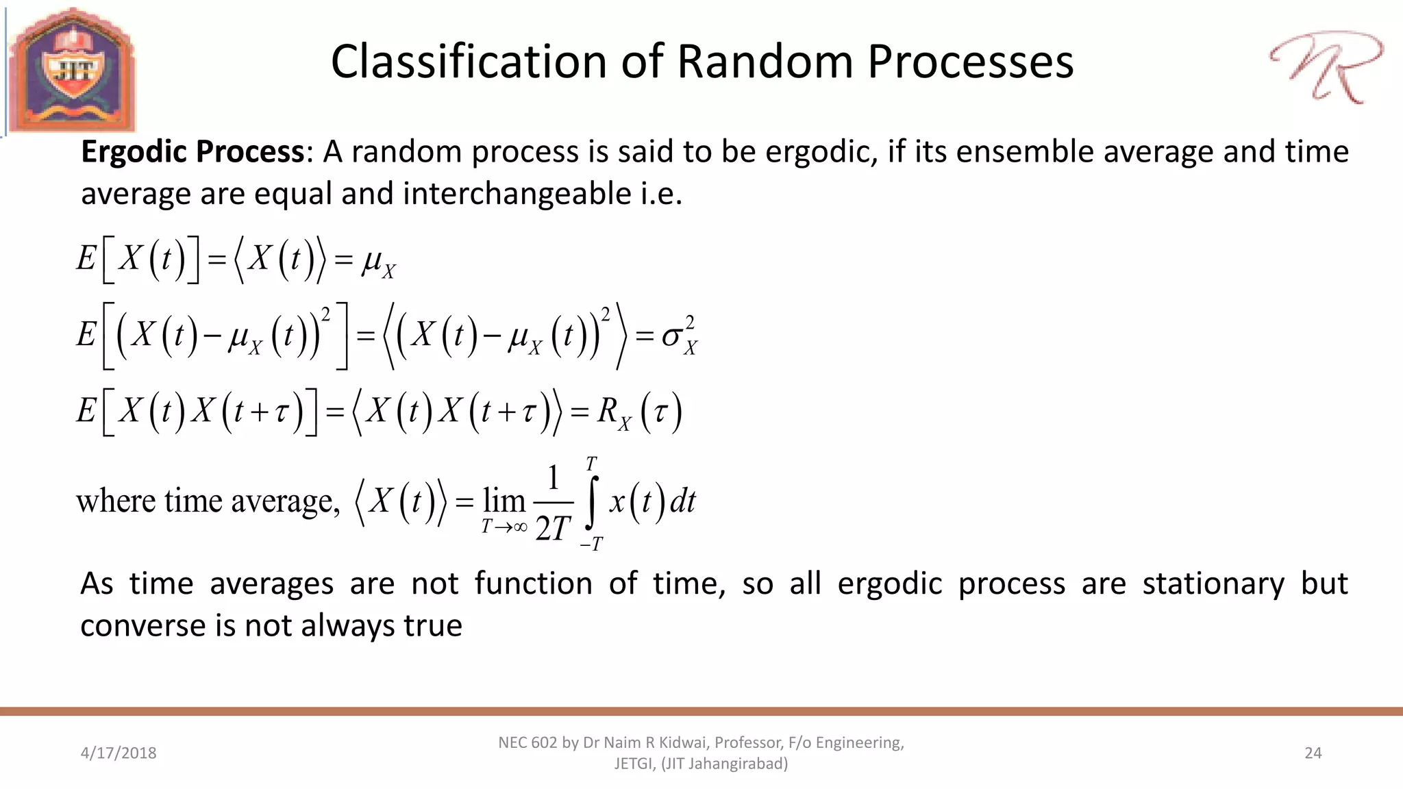
Ergodic Process: A random process is said to be ergodic, if its ensemble average and time
average are equal and interchangeable i.e.
   
         
         
   
2 2 2
1
where time average, lim
2
X
X X X
X
T
T
T
E X t X t
E X t t X t t
E X t X t X t X t R
X t x t dt
T

  
  


   
    
 
     
 
As time averages are not function of time, so all ergodic process are stationary but
converse is not always true

4/17/2018 25
   
     
         
      
2 2
2
2 2 2
2
2 2 2
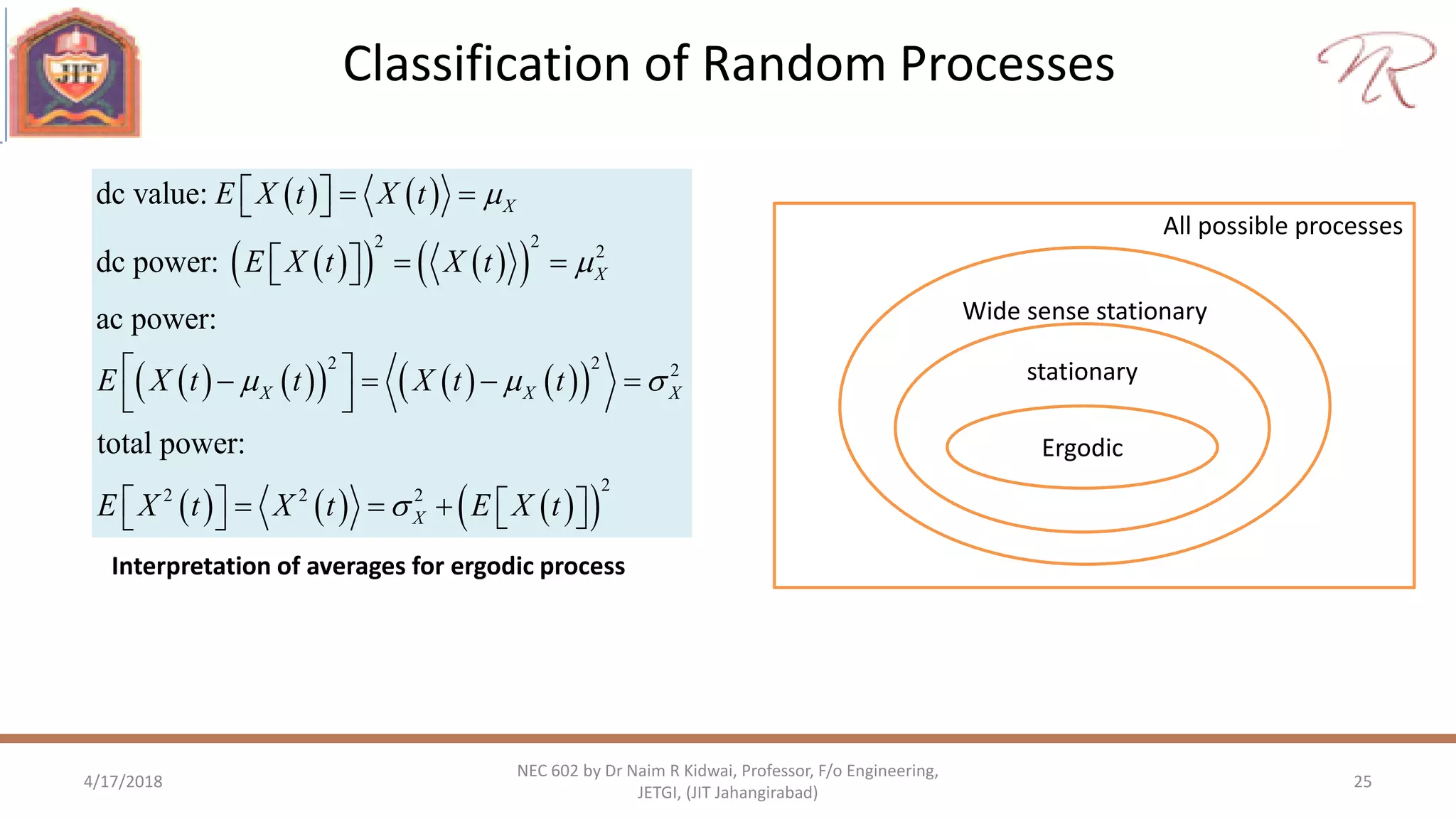
dc value:
dc power:
ac power:
total power:
X
X
X X X
X
E X t X t
E X t X t
E X t t X t t
E X t X t E X t


  

   
   
    
 
        
Interpretation of averages for ergodic process
All possible processes
Wide sense stationary
stationary
Ergodic

Power spectral density of WSS process
4/17/2018 26
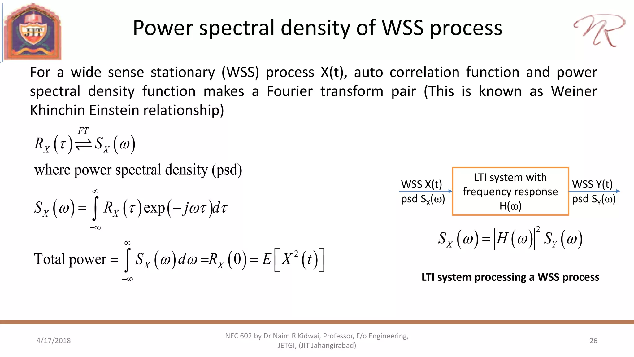
For a wide sense stationary (WSS) process X(t), auto correlation function and power
spectral density function makes a Fourier transform pair (This is known as Weiner
Khinchin Einstein relationship)
   
     
     2
where power spectral density (psd)
exp
Total power 0
FT
X X
X X
X X
R S
S R j d
S d R E X t
 
   
 




 
     


LTI system with
frequency response
H()
WSS X(t)
psd SX()
WSS Y(t)
psd SY()
     
2
X YS H S  
LTI system processing a WSS process

Multiple Random Processes
4/17/2018 27
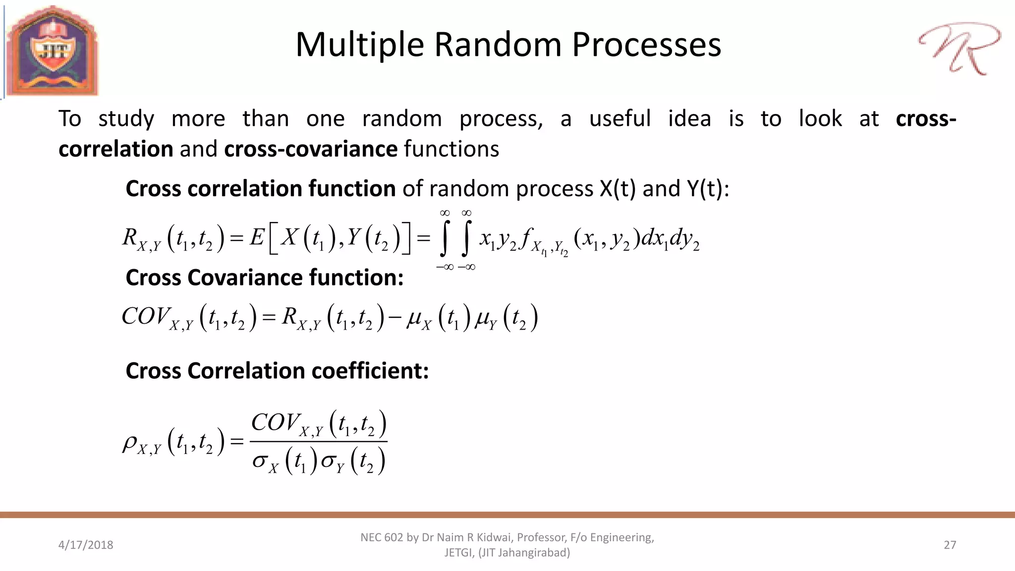
To study more than one random process, a useful idea is to look at cross-
correlation and cross-covariance functions
Cross correlation function of random process X(t) and Y(t):
       , 1 2 , 1 2 1 2, ,X Y X Y X YCOV t t R t t t t  
Cross Covariance function:
 
 
   
, 1 2
, 1 2
1 2
,
, X Y
X Y
X Y
COV t t
t t
t t

 

Cross Correlation coefficient:
      1 2
, 1 2 1 2 1 2 , 1 2 1 2, , ( , )t tX Y X YR t t E X t Y t x y f x y dx dy
 
 
     

Nec 602 unit ii Random Variables and Random process

More Related Content

What's hot

Similar to Nec 602 unit ii Random Variables and Random process

More from Dr Naim R Kidwai

Recently uploaded

In this document

Nec 602 unit ii Random Variables and Random process