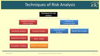
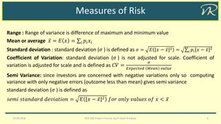
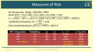
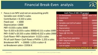
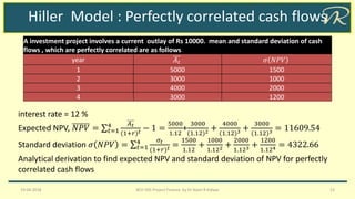
Project: Risk Analysis
19-04-2018 BCH 505 Project Finance by Dr Naim R Kidwai 1
Risk Analysis
▪ Risk is inherent in almost every business decision
▪ Risk refers to variability
▪ Capital budgeting decision involves cost and benefits over a long period of time
▪ Financial analysis has two phases
▪ feasibility analysis
▪ Risk analysis
▪ Sources of Risk
▪ Project Specific Risk: factors specific to project like quality, production
▪ Corporate Risk: action of competitors
▪ Industry specific Risk: technological developments and regulatory charges
▪ Market risk: Changes in microeconomic factors have impact project
▪ International risk: in case of foreign projects or political risk
19-04-2018 BCH 505 Project Finance by Dr Naim R Kidwai 2
Techniques of Risk Analysis
19-04-2018 BCH 505 Project Finance by Dr Naim R Kidwai 3
Techniques for risk
analysis
Analysis of Stand
alone Project
Analysis of
Contextual Risk
Sensitivity Analysis Scenario Analysis
Break Even Analysis Hillier Model
Simulation Analysis Decision tree analysis
Corporate Risk
Analysis
Market Risk Analysis
Measures of Risk
19-04-2018 BCH 505 Project Finance by Dr Naim R Kidwai 4
Range : Range of variance is difference of maximum and minimum value
Mean or average ҧ𝑥 = 𝐸 𝑥 = σ𝑖 𝑝𝑖 𝑥𝑖
Standard deviation : standard deviation (𝜎 ) is defined as 𝜎 = 𝐸 𝑥 − ҧ𝑥 2 = σ𝑖 𝑝𝑖 𝑥 − ҧ𝑥 2
Coefficient of Variation: standard deviation (𝜎 ) is not adjusted for scale. Coefficient of
variation is adjusted for scale and is defined as 𝐶𝑉 =
𝜎
𝐸𝑥𝑝𝑒𝑐𝑡𝑒𝑑 𝑀𝑒𝑎𝑛 𝑣𝑎𝑙𝑢𝑒
Semi Variance: since investors are concerned with negative variations only so computing
variance with only negative errors (outcome less than mean) gives semi variance
standard deviation (𝜎 ) is defined as
𝑠𝑒𝑚𝑖 𝑠𝑡𝑎𝑛𝑑𝑎𝑟𝑑 𝑑𝑒𝑣𝑖𝑎𝑡𝑖𝑜𝑛 = 𝐸 𝑥 − ҧ𝑥 2 𝑓𝑜𝑟 𝑜𝑛𝑙𝑦 𝑣𝑎𝑙𝑢𝑒𝑠 𝑜𝑓 𝑥 < ҧ𝑥
Measures of Risk
19-04-2018 BCH 505 Project Finance by Dr Naim R Kidwai 5
NPY ( thousands) x Probability p px x- ҧ𝑥 𝑥 − ҧ𝑥 2 p * sq. error
200 0.3 60 -340 115600 34680
600 0.5 300 60 3600 1800
900 0.2 180 360 129600 25920
mean NPV ( ҧ𝑥) 540 Sq. variance 62400
std deviation 249.8
For the example, Range = 900-200 = 700 K
𝑀𝑒𝑎𝑛 𝑁𝑃𝑉 = 0.3 𝑥 200 + 0.5 𝑥 600 + 0.2 𝑥900 = 540
𝜎 = 𝐸 𝑥 − ҧ𝑥 2 = 0.3 𝑥 (−340)2+0.5 𝑥 602 + 0.2 𝑥 3602 = 249.8 𝐾
Coefficient of Variation, 𝐶𝑉 =
249.8
540
= 0.46
Semi standard deviation= 0.3 𝑥 (−340)2= 186.2 𝐾
Measures of Risk
19-04-2018 BCH 505 Project Finance by Dr Naim R Kidwai 6
• Standard deviation is most commonly employed as measure of risk in finance.
• For computing mean and dispersion variables, probability distribution is required,
• If sufficient records for similar ventures are available, probability distribution is quite
‘objective,
• If sufficient records are not available, probability distribution is quite ‘subjective’,
Prospective on risk
There are three perspectives of the risk
• Stand alone risk: risk of the project when viewed in isolation
• Firm risk or Corporate risk: contribution of a project to the risk of the firm
• Systematic risk or market risk: risk of a project from view point of diversified investor
Sensitivity analysis
19-04-2018 BCH 505 Project Finance by Dr Naim R Kidwai 7
Sensitivity analysis is ‘what if’ analysis
NPV = -20000+4000 x PVIFA
= -20000+4000 x 5.65
= 2600 K
Cash flows depends on various factors and can
vary widely.
So optimistic and pessimistic estimates for
variables defined and NPV calculated
Cash Flow of ABC LTD project
(in thousands) Year 0 year 1-10
1 Investment 20000
2 Sales 18000
3 Variable cost ( 2/3 of sales) 12000
4 Fixed cost 1000
5 Depreciation 2000
6 Pre tax profit 3000
7 Taxes (@ 33.3 %) 1000
8 PAT 2000
9
cash flow from operation
(PAT+ depreciation) 4000
10 Net cash flow 2000 4000
Cost of capital 12%
Accumulated PV indexing factor (PVIFA) @12% 5.65
Sensitivity analysis
19-04-2018 BCH 505 Project Finance by Dr Naim R Kidwai 8
• NPV calculated by varying one variable at a time
• NPV is more sensitive to sales and least sensitive to fixed cost. For more sensitive
variable, it may be explored how variability of the factor can be contained.
• In real situation, many variable may change at a time so interpretation of results is
subjective
Sensitivity of NPV to variations in the value of key variables in ABC LTD project
Range (in thousands) NPV
Pessimistic Expected Optimistic Pessimistic Expected Optimistic Variation
1 Investment 24000 20000 18000 -1400 2600 4600 6000
2 Sales 15000 18000 21000 -1147 2600 6366 7513
3
Variable cost
as percentage
70 66.67 65 340 2600 3730 3390
4 Fixed cost 1300 1000 800 1470 2600 3353 1883
Scenario analysis
19-04-2018 BCH 505 Project Finance by Dr Naim R Kidwai 9
• Scenario analysis is beneficial when
various scenarios are well defined. It
considers several variable at a time
• More variable are required to be
estimated
• Normally scenarios are not discretely
defined
Sensitivity of NPV to variations in the value of key
variables in ABC LTD project
Range (in thousands)
Pessimistic Expected Optimistic
1 Investment 24000 20000 18000
2 Sales 15000 18000 21000
3
Variable cost
as percentage
70 66.67 65
4 Fixed cost 1300 1000 800
NPV -8180 2600 10438
Break-Even analysis
19-04-2018 BCH 505 Project Finance by Dr Naim R Kidwai 10
• It tells what is minimum value of key variables/
revenues so that project does not ‘lose money’
• Variable cost to sales ratio= 12/18= 0.667
• Contribution to margin ratio =0.333
• Accounting break even=
𝐹𝑖𝑥𝑒𝑑 𝑐𝑜𝑠𝑡+𝑑𝑒𝑝𝑟𝑒𝑐𝑖𝑎𝑡𝑖𝑜𝑛
𝑐𝑜𝑛𝑡𝑟𝑖𝑏𝑢𝑡𝑖𝑜𝑛 𝑡𝑜 𝑚𝑎𝑟𝑔𝑖𝑛 𝑟𝑎𝑡𝑖𝑜
=
1000+2000
0.333
= 9000 𝐾
• For sales 0f 9000 K , PBT, PAT will be zero
• At accounting break even project gives zero %
return
Cash Flow of ABC LTD project
(in thousands) Year 0 year 1-10
1 Investment 20000
2 Sales 18000
3 Variable cost ( 2/3 of sales) 12000
4 Fixed cost 1000
5 Depreciation 2000
6 Pre tax profit 3000
7 Taxes (@ 33.3 %) 1000
8 PAT 2000
9
cash flow from operation
(PAT+ depreciation) 4000
10 Net cash flow 2000 4000
Cost of capital 12%
Accumulated PV indexing factor (PVIFA) @ 12 % 5.65
Financial Break-Even analysis
19-04-2018 BCH 505 Project Finance by Dr Naim R Kidwai 11
• Focus is on NPV and not on accounting profit
Variable cost =0.667 x sales
Contribution = 0.333 x sales
Fixed cost = 1000
Depreciation =2000
PBT= 0.333 x sales-3000
Tax= 0.333 x (0.333 x sales-3000)=0.111 x sales-1000
PAT= 0.667 x (0.333 x sales-3000)=0.222 x sales-2000
Cash flows= PAT+ depreciation= 0.222 x sales
PV of cash flows= Cash flows x PVIFA= 1.255 x sales
Breakeven NPV = 20000- 1.255 x sales= 0
so Breakeven sales= 15936 K
Cash Flow of ABC LTD project
(in thousands) Year 0 year 1-10
1 Investment 20000
2 Sales 18000
3 Variable cost (2/3 of sales) 12000
4 Fixed cost 1000
5 Depreciation 2000
6 Pre tax profit 3000
7 Taxes (@ 33.3 %) 1000
8 PAT 2000
9
cash flow from operation
(PAT+ depreciation) 4000
10 Net cash flow 2000 4000
Cost of capital 12%
Accumulated PV indexing factor (PVIFA) @ 12% 5.65
Hiller Model : Un correlated cash flows
19-04-2018 BCH 505 Project Finance by Dr Naim R Kidwai 12
interest rate = 12 %
Expected NPV, 𝑁𝑃𝑉 = σ 𝑡=1
3 𝐴 𝑡
(1+𝑟) 𝑡 =
5000
1.12
+
4000
(1.12)2 +
5000
(1.12)3
= 4464.3 + 3188. 8 + 3558.9 = 11211.9
Standard deviation 𝜎 𝑁𝑃𝑉 = σ 𝑡=1
3 𝜎𝑡
2
(1+𝑟)2𝑡 =
2400000
1.122 +
1600000
1.124 +
2400000
1.126 = 2036.18
Analytical derivation to find expected NPV and standard deviation of NPV
Year 1 Year 2 Year 3
Net Cash flow (Rs) Probability Net Cash flow (Rs) Probability Net Cash flow (Rs) Probability
3000 0.3 2000 0.2 3000 0.3
5000 0.4 4000 0.6 5000 0.4
7000 0.3 6000 0.2 7000 0.3
Mean 5000 4000 5000
Standard variance 2400000 Standard variance 1600000 Standard variance 2400000
Hiller Model : Perfectly correlated cash flows
19-04-2018 BCH 505 Project Finance by Dr Naim R Kidwai 13
interest rate = 12 %
Expected NPV, 𝑁𝑃𝑉 = σ 𝑡=1
4 𝐴 𝑡
(1+𝑟) 𝑡 − 1 =
5000
1.12
+
3000
(1.12)2 +
4000
(1.12)3 +
3000
(1.12)3 = 11609.54
Standard deviation 𝜎 𝑁𝑃𝑉 = σ 𝑡=1
4 𝜎𝑡
(1+𝑟) 𝑡 =
1500
1.12
+
1000
1.122 +
2000
1.123 +
1200
1.124 = 4322.66
Analytical derivation to find expected NPV and standard deviation of NPV for perfectly
correlated cash flows
A investment project involves a current outlay of Rs 10000. mean and standard deviation of cash
flows , which are perfectly correlated are as follows
year 𝐴 𝑡 𝜎 𝑁𝑃𝑉
1 5000 1500
2 3000 1000
3 4000 2000
4 3000 1200
Simulation Analysis
19-04-2018 BCH 505 Project Finance by Dr Naim R Kidwai 14
• Sensitivity of criterion of merit (NPV IRR, ROI etc.) may not be adequate for decision making
• Likelihood of occurrence of circumstances (probability profile) can be obtained by
simulation
• The steps in simulation analysis are (criterion of merit is NPV)
1. Model the project : how criterion of merit is related to variables
• Parameter variables : input variables given by decision maker held constant in
simulation
• Exogenous variable: which are random in nature and can not be controlled
2. Specify the value of parameters and probability distribution of exogenous variables
3. Select a value randomly from probability distribution of exogenous variables.
4. Determine NPV
5. Repeat steps 2 to 4 a number of times to get large number of simulated NPV’s
6. Plot the frequency distribution of NPV
Project selection under risk
19-04-2018 BCH 505 Project Finance by Dr Naim R Kidwai 15
• Judgemental Evaluation: Accept or reject the project based on the risk and return
characteristics without any formal method for incorporating risk in decision making
• Payback period requirement: payback period requirement is applied to control risk.
• Risk adjusted discount method:
• If the risk of the project is equal to risk of existing investment, discount rate is
average cost of capital
• If the risk of the project is greater than risk of existing investment, discount rate is
higher than average cost of capital
Thank You
19-04-2018 BCH 505 Project Finance by Dr Naim R Kidwai 16
Contact
Email: naimkidwai@gmail.com
https://nrkidwai.wordpress.com/

project risk analysis

  • 1.
    Project: Risk Analysis 19-04-2018BCH 505 Project Finance by Dr Naim R Kidwai 1
  • 2.
    Risk Analysis ▪ Riskis inherent in almost every business decision ▪ Risk refers to variability ▪ Capital budgeting decision involves cost and benefits over a long period of time ▪ Financial analysis has two phases ▪ feasibility analysis ▪ Risk analysis ▪ Sources of Risk ▪ Project Specific Risk: factors specific to project like quality, production ▪ Corporate Risk: action of competitors ▪ Industry specific Risk: technological developments and regulatory charges ▪ Market risk: Changes in microeconomic factors have impact project ▪ International risk: in case of foreign projects or political risk 19-04-2018 BCH 505 Project Finance by Dr Naim R Kidwai 2
  • 3.
    Techniques of RiskAnalysis 19-04-2018 BCH 505 Project Finance by Dr Naim R Kidwai 3 Techniques for risk analysis Analysis of Stand alone Project Analysis of Contextual Risk Sensitivity Analysis Scenario Analysis Break Even Analysis Hillier Model Simulation Analysis Decision tree analysis Corporate Risk Analysis Market Risk Analysis
  • 4.
    Measures of Risk 19-04-2018BCH 505 Project Finance by Dr Naim R Kidwai 4 Range : Range of variance is difference of maximum and minimum value Mean or average ҧ𝑥 = 𝐸 𝑥 = σ𝑖 𝑝𝑖 𝑥𝑖 Standard deviation : standard deviation (𝜎 ) is defined as 𝜎 = 𝐸 𝑥 − ҧ𝑥 2 = σ𝑖 𝑝𝑖 𝑥 − ҧ𝑥 2 Coefficient of Variation: standard deviation (𝜎 ) is not adjusted for scale. Coefficient of variation is adjusted for scale and is defined as 𝐶𝑉 = 𝜎 𝐸𝑥𝑝𝑒𝑐𝑡𝑒𝑑 𝑀𝑒𝑎𝑛 𝑣𝑎𝑙𝑢𝑒 Semi Variance: since investors are concerned with negative variations only so computing variance with only negative errors (outcome less than mean) gives semi variance standard deviation (𝜎 ) is defined as 𝑠𝑒𝑚𝑖 𝑠𝑡𝑎𝑛𝑑𝑎𝑟𝑑 𝑑𝑒𝑣𝑖𝑎𝑡𝑖𝑜𝑛 = 𝐸 𝑥 − ҧ𝑥 2 𝑓𝑜𝑟 𝑜𝑛𝑙𝑦 𝑣𝑎𝑙𝑢𝑒𝑠 𝑜𝑓 𝑥 < ҧ𝑥
  • 5.
    Measures of Risk 19-04-2018BCH 505 Project Finance by Dr Naim R Kidwai 5 NPY ( thousands) x Probability p px x- ҧ𝑥 𝑥 − ҧ𝑥 2 p * sq. error 200 0.3 60 -340 115600 34680 600 0.5 300 60 3600 1800 900 0.2 180 360 129600 25920 mean NPV ( ҧ𝑥) 540 Sq. variance 62400 std deviation 249.8 For the example, Range = 900-200 = 700 K 𝑀𝑒𝑎𝑛 𝑁𝑃𝑉 = 0.3 𝑥 200 + 0.5 𝑥 600 + 0.2 𝑥900 = 540 𝜎 = 𝐸 𝑥 − ҧ𝑥 2 = 0.3 𝑥 (−340)2+0.5 𝑥 602 + 0.2 𝑥 3602 = 249.8 𝐾 Coefficient of Variation, 𝐶𝑉 = 249.8 540 = 0.46 Semi standard deviation= 0.3 𝑥 (−340)2= 186.2 𝐾
  • 6.
    Measures of Risk 19-04-2018BCH 505 Project Finance by Dr Naim R Kidwai 6 • Standard deviation is most commonly employed as measure of risk in finance. • For computing mean and dispersion variables, probability distribution is required, • If sufficient records for similar ventures are available, probability distribution is quite ‘objective, • If sufficient records are not available, probability distribution is quite ‘subjective’, Prospective on risk There are three perspectives of the risk • Stand alone risk: risk of the project when viewed in isolation • Firm risk or Corporate risk: contribution of a project to the risk of the firm • Systematic risk or market risk: risk of a project from view point of diversified investor
  • 7.
    Sensitivity analysis 19-04-2018 BCH505 Project Finance by Dr Naim R Kidwai 7 Sensitivity analysis is ‘what if’ analysis NPV = -20000+4000 x PVIFA = -20000+4000 x 5.65 = 2600 K Cash flows depends on various factors and can vary widely. So optimistic and pessimistic estimates for variables defined and NPV calculated Cash Flow of ABC LTD project (in thousands) Year 0 year 1-10 1 Investment 20000 2 Sales 18000 3 Variable cost ( 2/3 of sales) 12000 4 Fixed cost 1000 5 Depreciation 2000 6 Pre tax profit 3000 7 Taxes (@ 33.3 %) 1000 8 PAT 2000 9 cash flow from operation (PAT+ depreciation) 4000 10 Net cash flow 2000 4000 Cost of capital 12% Accumulated PV indexing factor (PVIFA) @12% 5.65
  • 8.
    Sensitivity analysis 19-04-2018 BCH505 Project Finance by Dr Naim R Kidwai 8 • NPV calculated by varying one variable at a time • NPV is more sensitive to sales and least sensitive to fixed cost. For more sensitive variable, it may be explored how variability of the factor can be contained. • In real situation, many variable may change at a time so interpretation of results is subjective Sensitivity of NPV to variations in the value of key variables in ABC LTD project Range (in thousands) NPV Pessimistic Expected Optimistic Pessimistic Expected Optimistic Variation 1 Investment 24000 20000 18000 -1400 2600 4600 6000 2 Sales 15000 18000 21000 -1147 2600 6366 7513 3 Variable cost as percentage 70 66.67 65 340 2600 3730 3390 4 Fixed cost 1300 1000 800 1470 2600 3353 1883
  • 9.
    Scenario analysis 19-04-2018 BCH505 Project Finance by Dr Naim R Kidwai 9 • Scenario analysis is beneficial when various scenarios are well defined. It considers several variable at a time • More variable are required to be estimated • Normally scenarios are not discretely defined Sensitivity of NPV to variations in the value of key variables in ABC LTD project Range (in thousands) Pessimistic Expected Optimistic 1 Investment 24000 20000 18000 2 Sales 15000 18000 21000 3 Variable cost as percentage 70 66.67 65 4 Fixed cost 1300 1000 800 NPV -8180 2600 10438
  • 10.
    Break-Even analysis 19-04-2018 BCH505 Project Finance by Dr Naim R Kidwai 10 • It tells what is minimum value of key variables/ revenues so that project does not ‘lose money’ • Variable cost to sales ratio= 12/18= 0.667 • Contribution to margin ratio =0.333 • Accounting break even= 𝐹𝑖𝑥𝑒𝑑 𝑐𝑜𝑠𝑡+𝑑𝑒𝑝𝑟𝑒𝑐𝑖𝑎𝑡𝑖𝑜𝑛 𝑐𝑜𝑛𝑡𝑟𝑖𝑏𝑢𝑡𝑖𝑜𝑛 𝑡𝑜 𝑚𝑎𝑟𝑔𝑖𝑛 𝑟𝑎𝑡𝑖𝑜 = 1000+2000 0.333 = 9000 𝐾 • For sales 0f 9000 K , PBT, PAT will be zero • At accounting break even project gives zero % return Cash Flow of ABC LTD project (in thousands) Year 0 year 1-10 1 Investment 20000 2 Sales 18000 3 Variable cost ( 2/3 of sales) 12000 4 Fixed cost 1000 5 Depreciation 2000 6 Pre tax profit 3000 7 Taxes (@ 33.3 %) 1000 8 PAT 2000 9 cash flow from operation (PAT+ depreciation) 4000 10 Net cash flow 2000 4000 Cost of capital 12% Accumulated PV indexing factor (PVIFA) @ 12 % 5.65
  • 11.
    Financial Break-Even analysis 19-04-2018BCH 505 Project Finance by Dr Naim R Kidwai 11 • Focus is on NPV and not on accounting profit Variable cost =0.667 x sales Contribution = 0.333 x sales Fixed cost = 1000 Depreciation =2000 PBT= 0.333 x sales-3000 Tax= 0.333 x (0.333 x sales-3000)=0.111 x sales-1000 PAT= 0.667 x (0.333 x sales-3000)=0.222 x sales-2000 Cash flows= PAT+ depreciation= 0.222 x sales PV of cash flows= Cash flows x PVIFA= 1.255 x sales Breakeven NPV = 20000- 1.255 x sales= 0 so Breakeven sales= 15936 K Cash Flow of ABC LTD project (in thousands) Year 0 year 1-10 1 Investment 20000 2 Sales 18000 3 Variable cost (2/3 of sales) 12000 4 Fixed cost 1000 5 Depreciation 2000 6 Pre tax profit 3000 7 Taxes (@ 33.3 %) 1000 8 PAT 2000 9 cash flow from operation (PAT+ depreciation) 4000 10 Net cash flow 2000 4000 Cost of capital 12% Accumulated PV indexing factor (PVIFA) @ 12% 5.65
  • 12.
    Hiller Model :Un correlated cash flows 19-04-2018 BCH 505 Project Finance by Dr Naim R Kidwai 12 interest rate = 12 % Expected NPV, 𝑁𝑃𝑉 = σ 𝑡=1 3 𝐴 𝑡 (1+𝑟) 𝑡 = 5000 1.12 + 4000 (1.12)2 + 5000 (1.12)3 = 4464.3 + 3188. 8 + 3558.9 = 11211.9 Standard deviation 𝜎 𝑁𝑃𝑉 = σ 𝑡=1 3 𝜎𝑡 2 (1+𝑟)2𝑡 = 2400000 1.122 + 1600000 1.124 + 2400000 1.126 = 2036.18 Analytical derivation to find expected NPV and standard deviation of NPV Year 1 Year 2 Year 3 Net Cash flow (Rs) Probability Net Cash flow (Rs) Probability Net Cash flow (Rs) Probability 3000 0.3 2000 0.2 3000 0.3 5000 0.4 4000 0.6 5000 0.4 7000 0.3 6000 0.2 7000 0.3 Mean 5000 4000 5000 Standard variance 2400000 Standard variance 1600000 Standard variance 2400000
  • 13.
    Hiller Model :Perfectly correlated cash flows 19-04-2018 BCH 505 Project Finance by Dr Naim R Kidwai 13 interest rate = 12 % Expected NPV, 𝑁𝑃𝑉 = σ 𝑡=1 4 𝐴 𝑡 (1+𝑟) 𝑡 − 1 = 5000 1.12 + 3000 (1.12)2 + 4000 (1.12)3 + 3000 (1.12)3 = 11609.54 Standard deviation 𝜎 𝑁𝑃𝑉 = σ 𝑡=1 4 𝜎𝑡 (1+𝑟) 𝑡 = 1500 1.12 + 1000 1.122 + 2000 1.123 + 1200 1.124 = 4322.66 Analytical derivation to find expected NPV and standard deviation of NPV for perfectly correlated cash flows A investment project involves a current outlay of Rs 10000. mean and standard deviation of cash flows , which are perfectly correlated are as follows year 𝐴 𝑡 𝜎 𝑁𝑃𝑉 1 5000 1500 2 3000 1000 3 4000 2000 4 3000 1200
  • 14.
    Simulation Analysis 19-04-2018 BCH505 Project Finance by Dr Naim R Kidwai 14 • Sensitivity of criterion of merit (NPV IRR, ROI etc.) may not be adequate for decision making • Likelihood of occurrence of circumstances (probability profile) can be obtained by simulation • The steps in simulation analysis are (criterion of merit is NPV) 1. Model the project : how criterion of merit is related to variables • Parameter variables : input variables given by decision maker held constant in simulation • Exogenous variable: which are random in nature and can not be controlled 2. Specify the value of parameters and probability distribution of exogenous variables 3. Select a value randomly from probability distribution of exogenous variables. 4. Determine NPV 5. Repeat steps 2 to 4 a number of times to get large number of simulated NPV’s 6. Plot the frequency distribution of NPV
  • 15.
    Project selection underrisk 19-04-2018 BCH 505 Project Finance by Dr Naim R Kidwai 15 • Judgemental Evaluation: Accept or reject the project based on the risk and return characteristics without any formal method for incorporating risk in decision making • Payback period requirement: payback period requirement is applied to control risk. • Risk adjusted discount method: • If the risk of the project is equal to risk of existing investment, discount rate is average cost of capital • If the risk of the project is greater than risk of existing investment, discount rate is higher than average cost of capital
  • 16.
    Thank You 19-04-2018 BCH505 Project Finance by Dr Naim R Kidwai 16 Contact Email: naimkidwai@gmail.com https://nrkidwai.wordpress.com/