SlideShare a Scribd company logo
1 of 64
1
Chapter 6
Sampling and Analog-to-
Digital Conversion
2
Content
1. Sampling Theorem
2. Pulse Code Modulation (PCM)
3. Digital Telephony: PCM in T1 Carrier Systems
4. Digital Multiplexing
5. Differential Pulse Code Modulation (DPCM)
6. Adaptive DPCM (ADPCM)
7. Delta Modulation
3
6.1 Sampling Theorem
Significance
Analog signals can be digitized through sampling and
quantization. The sampling rate must be sufficiently
large so that the analog signal can be reconstructed
from the samples with sufficient accuracy. The sampling
theorem, which is the basis for determining the proper
sampling rate for a given signal, has a deep significance
in signal processing and communication theory.
4
6.1 Sampling Theorem
The theorem
Any signal whose spectrum is band-limited to B
Hz can be reconstructed exactly (without any
error) from its samples taken uniformly at a rate
fs >= 2B Hz (samples per second). In other
words, the minimum sampling frequency is:
fs = 2B Hz.
6.1 Sampling Theorem
To prove the sampling theorem, consider a
signal g(t) (Fig. 6.1 a) whose spectrum is band-
limited to B Hz (Fig. 6.1b). Sampling g(t) at a
rate of fs Hz can be accomplished by
multiplying g(t) by an impulse train δTs(t) (Fig.
6.1c), consisting of unit impulses repeating
periodically every Ts seconds, where Ts = 1/ fs.
6
6.1 Sampling Theorem
1/Ts
x
*
Figure 6.1 Sampled signal and its Fourier spectra.
1/Ts
           









n
t
f
jn
s
n
s
s
Ts
s
e
t
g
T
nT
t
nT
g
t
t
g
t
g 

 2
1
  





n
n
t
jn
s
Ts
s
e
T
t 

1
   






n
s
s
nf
f
G
T
f
G
1
7
6.1 Sampling Theorem
Since the impulse train Ts(t) is a periodic signal of period Ts , it can be expressed as a
Fourier series. Its exponential Fourier series is given by:
         
 


n
s
s
Ts nT
t
nT
g
t
t
g
t
g 

  





n
n
t
jn
s
Ts
s
e
T
t 

1
s
s
s f
T


 2
2


       






n
t
f
jn
s
T
s
s
e
t
g
T
t
t
g
t
g 
 2
1
Therefore
Taking the Fourier Transform:
   






n
s
s
nf
f
G
T
f
G
1
(Example 2.5 on page 45
of the text book)
(Example 3.5 on page 74 and Example 3.11 on page 86 of the text book )
If we are to reconstruct g(t) from ḡ(t), we should be
able to recover G( f ) from Ḡ ( f ) using a LPF. This is
possible if there is no overlap between successive cycles
of Ḡ ( f ). This requires fs > 2B. Since the sampling
interval is Ts=1/fs this implies
Therefore,
1
2
S
T
B

The minimum sampling rate fs > 2B samples/second
required to recover g(t) from its samples ḡ(t) is called
the Nyquist rate for g(t), and the corresponding sampling
interval Ts=1/(2B) seconds is called the
Nyquist Interval for g(t).
6.1 Sampling Theorem
9
Signal Reconstruction: The
Interpolation Formula
  







B
f
T
f
H s
2
The process of reconstructing a continuous-time signal g(t) from
its samples is also known as interpolation. A signal g(t) band-
limited to B Hz can be reconstructed (interpolated) exactly from
its samples. This is done by passing the sampled signal through
an ideal low-pass filter of bandwidth B Hz and gain Ts to recover
the component (1/Ts)g(t) from the sampled signal. Thus, the
reconstruction (or interpolating) filter transfer function is
   
Bt
BT
t
h s 
2
sinc
2

10
Signal Reconstruction: The Interpolation Formula
Assuming the Nyquist sampling rate, that is:
2B = fs = 1/Ts we obtain
h(t) = sinc(2πBt)
  







B
f
T
f
H s
2
   
Bt
BT
t
h s 
2
sinc
2

h(t) = sinc(2πBt)
11
Signal Reconstruction: The Interpolation Formula
The kth sample of the input ͞g(t) is the impulse g(nTs)δ(t-
nTs); the filter output of this impulse is g(nTs)h(t-nTs).
Hence the filter output ͞g(t), which is g(t), can now be
expressed as a sum,
     
   
 
   



n
Bt
nT
g
nT
t
B
nT
g
nT
t
h
nT
g
t
g
n
s
s
n
s
s
n
s









2
sinc
2
sinc
12
Signal Reconstruction: The Interpolation Formula
The above equation is the interpolation formula,
which yields values of g(t) between samples as a
weighted sum of all the sample values.
     

 n
Bt
nT
g
t
g
n
s 
  2
sinc
13
Practical Sampling
Practical Sampling
In proving the sampling theorem, we assumed ideal samples
obtained by multiplying a signal g(t) by an impulse train which is
physically nonexistent. In practice, we multiply a signal g(t) by a
train of pulses of finite width, shown in the next figure. We
wonder whether it is possible to recover or reconstruct g(t) from
the sampled signal. Surprisingly, the answer is positive, provided
that the sampling rate is not below the Nyquist rate. The signal
g(t) can be recovered by low-pass filtering the sampled signal as if
it were sampled by impulse train.
14
Practical Sampling
The envelope is FT of a pulse
x
*
Practical Sampling
                 
    






















n
t
f
jn
s
n
s
n
s
n
s
s
e
T
t
p
t
g
nT
t
t
p
t
g
nT
t
t
p
t
g
nT
t
p
t
g
t
g



2
1
*
*
*
~
       
     
   




















n
s
s
s
n
s
s
s
n
s
s
nf
f
G
nf
P
T
nf
f
nf
P
T
f
G
nf
f
T
f
P
f
G
f
G
1
1
~


Fourier Transform (spectrum) of the sampled signal is:
Therefore g(t) can by reconstructed using a low pass filter (LPF) of
B < Bandwidth < fs - B
16
Practical Sampling
               
t
g
t
p
nT
t
nT
g
t
p
nT
t
p
nT
g
t
g
n
s
s
n
s
s *
*
~ 



 
 
Therefore
     






n
s
s
nf
f
G
T
f
P
f
G
1
~
Nevertheless in practical scenarios scaling factor for
amplitude of each pulse can be considered a constant
value over the pulse duration. In this case sampled signal
Figure 6.5 Practical signal reconstruction.
17
Practical Sampling
The equalizer must remove all the shifted replicas
G( f - n fs) for n > 0
The sampling pulse can be approximated to rectangular pulses:
   









B
f
T
B
f
f
f
P
f
E
s
s
0
  






 


p
p
T
T
t
t
p
5
.
0
   
sin p
j fT
p p
P f T c fT e




To recover g(t) a filter (called equalizer) is needed. Let
E(f) is the frequency response of the equalizer such that
           







n
s
s
nf
f
G
T
f
P
f
E
f
G
f
E
f
G
1
~
18
Practical Sampling
As a result E( f ) must be :
 
 
 
 
















B
f
f
B
f
f
B
Flexible
B
f
f
P
T
f
E
s
s
s
0
 
  B
f
e
fT
f
T
f
E p
fT
j
p
s 


|
|
sin



By choosing Tp small:
  B
f
T
T
f
E
p
s

 |
|
19
Maximum Information Rate
A minimum of 2B independent pieces of information
per second can be transmitted, error free, over a
noiseless channel of bandwidth B Hz. This can be
proved by the sampling theorem.
20
Some Applications of the Sampling Theorem
Figure 6.11 Pulse-modulated signals. (a) The unmodulated signal. (b) The PAM signal.
(c) The PWM (PDM) signal. (d) The PPM signal.
21
Some Applications of the Sampling Theorem
Figure 6.12 Time division multiplexing of two signals.
22
6.2 Pulse Code Modulation
PCM is the most used among the pulse modulation
techniques. It is used to convert analog signal to digital
one.
After quantizing a sampled signal we obtain a L-level
pulse train. This signal can be converted to “binary
pulses” by assigning a binary code for each level. Thus
the L-ary signal is converted to a binary signal where
the 0 and 1 can be expressed as -1V and +1V.
Figure 6.13 PCM system diagram.
23
Quantization
Figure 6.14 Quantization of a sampled analog signal.
24
Quantization
25
Binary Code and Pulses
26
Pulse Code Modulation
Example1: telephony systems
Step1: the bandwidth is limited to 3400Hz (enough for
intelligibility) with low pass filter.
Step2: the resulting signal is sampled with fs = 8000Hz
(> 6.8KHz).
Step3: the samples are quantized to 256 levels = 28.
Step4: the quantized levels are then coded with 8-bit
binary code.  the telephone signal require a rate of
8000x 8 =64000 binary pulses per second (64kbps).
27
Pulse Code Modulation
Example2: compact disc CD
Step1: the bandwidth is limited to 15kHz, since it is a HIFI
system.
Step2: the resulting signal is sampled with fs = 44.1kHz
(> 30kHz).
Step3: the samples are quantized to 65,536 levels = 216.
Step4: the quantized levels are then coded with 16-bit
binary code.  the binary pulses are then recorded in the
CD
28
2.2 Uniform Quantizing
Figure 6.14 Quantization of a sampled analog signal.
29
2.2 Uniform Quantizing
In digital communication, the detection error is usually
much less than the quantizing error and can be ignored
i.e., the detection error is ignored.
For quantizing, we limit the amplitude of the message
signal m(t) to the range (-mp, mp), as shown in Fig. 6.10.
Note that mp is not necessarily the peak amplitude of m(t).
The amplitudes of m(t) beyond ±mp are chopped off. Thus,
mp is not a parameter of the signal m(t), but is a constant of
the quantizer. The amplitude range (-mp, mp) is divided into
L uniformly spaced intervals, each of width
Δv = 2mp/L.
(a) Quantizer characteristic of a uniform quantizer (b) Error signal
v v v v
v
v
v
v
v/2
v/2
v/2
v/2
v/2
v/2
v/2
v/2
Quantizer
Input x
Quantizer
Output xq
q
x
x
mp
v v v v
v
v
v
v
v/2
Quantizer
Input x
Quantization Error q
v/2
mp
(a)
(b)
Quantizing Error (noise)
Uniform Quantizer
Δv = 2mp/L = x-xq
Example:
A signal m(t) with amplitude variations in the range -mp to
mp is to be sent using PCM with a uniform quantizer. The
quantization error should be less than or equal to 0.1
percent of the peak value mp. If the signal is band limited
to 5 kHz, find the minimum bit rate required by this
scheme.
Ans: 105 bps
32
Quantizing Noise
The mean square of the original signal is:  
t
m
S 2
0 
The mean square of the quantization error is: 2
2
2
0
3
12 L
m
v
N
p



Where L, number of the quantizer levels and mp is the
highest quantizer level. (a constant of the quantizer)
The SNR, signal to noise ratio is given by:
 
2
2
2
0
0
3
p
m
t
m
L
N
S
SNR 

Δv = 2mp/L
33
2.3 Non-uniform Quantizing
Normally we prefer a constant SNR. Unfortunately it is
not the case. The SNR is directly related to the mean
power of the signal varying from one talker to another.
They also vary with the path length. This is due to the
fact that the quantizer step is constant v = 2mp / L. The
quantizing error is directly proportional to the step size.
How to maintain a constant SNR for different signals?
34
Non-uniform Quantizing
Solution
 Taking smaller steps for small signals and larger steps for large
signals.  nonuniform quantizing.
 Same result can be obtained by signal compression followed by
quantization with uniform-step quantizer
e.g. logarithmic compression
Compression function
35
Non-uniform Quantizing
smaller quantization noise for small signal.
SNR independent from the signal power for
large dynamic range
 disadvantage: more noise in strong signals.
36
Non-uniform Quantizing
  










p
m
m
y


1
ln
1
ln
1
1
0 

p
m
m
 
 































1
1
1
ln
ln
1
1
1
0
ln
ln
1
1
p
p
p
p
m
m
A
m
Am
A
A
m
m
m
m
A
y
Compression laws:
law (in North America and Japan)
Alaw (In Europe and the rest of the world)
37
Non-uniform Quantizing
38
Non-uniform Quantizing
The coefficients  or A define the degree of
compression.
 For 128-level (7 bits) encoding,  = 100 is used
leading to a dynamic range of 40dB.
 For 256-level (8 bits) encoding,  = 255 is used
leading to a dynamic range of 40dB.
 For 256-level (8 bits) encoding, A = 87.6 is used
leading to a comparable results.
• A number of companies manufacture CODEC chips with various
specifications and in various configurations. Some of these
companies are:
Motorola (USA), National semiconductors (USA), OKI (Japan).
• These ICs include the anti-aliasing bandpass filter (300 Hz to 3.4
kHz), receiver lowpass filter, pin selectable A-law / μ -law option.
Listed below are some of the chip numbers manufactured by
these companies.
Motorola: MC145500 to MC145505
National: TP3070, TP3071 and TP3070-X
OKI: MSM7578H / 7578V / 7579
Details about these ICs can be downloaded from their respective websites.
40
Non-uniform Quantizing
At the receiver end an expander must be used to
restore the original signal. The compressor and the
expander are together called the compander.
In  -law compander the SNR is found to be:
 
   
t
m
m
for
L
N
S p
2
2
2
2
2
0
0
~
1
ln
3


 

41
Non-uniform Quantizing
42
Non-uniform Quantizing
Compander
Based on logarithmic diode characteristics.










s
I
I
q
KT
V 1
ln
Encoder and Decoder
 Sampling, quantization and encoding are performed
using the Analog to Digital Converter
 Digital to Analog Converter can be used for
decoding.
43
Comments on Logarithmic Units
(Decibel)
 Voltage: V = x Volt  VdB = 20log10(x).
 Ratio between voltages:
A = V1/V2  AdB = 20log10(A).
 Power: P = y Watt  PdB = 10log10(y).
P = y mWatt  PdBm = 10log10(y).
PdBm = PdB + 30
 Ratio between Powers:
G = P1/P2 =  GdB = 10log10(G).
44
Pulse Code Modulation
45
2.3 Transmission Bandwidth and
the Output SNR
For a binary PCM, we assign a distinct group of n binary digits (bits)
to each of the L quantization levels. Because a sequence of n binary
digits can be arranged in 2n distinct patterns,
L = 2n or n = log2 L (6.37)
Each quantized sample is, thus, encoded into n bits. Because a
signal m(t) band-limited to B Hz requires a minimum of 2B samples
per second, we require a total of 2nB bits per second (bps), that is,
2nB pieces of information per second. Because a unit bandwidth (1
Hz) can transmit a maximum of two pieces of information per
second, we require a minimum channel of bandwidth BT Hz, given
by
BT = nB Hz (6.38)
46
Pulse Code Modulation
(6.37)
(6.40)
(6.39)
(6.41)
(6.34) (6.36)
(6.34)
(6.36)
(6.38) (6.39)
(6.40)
47
Pulse Code Modulation
48
Digital Telephony: PCM in T1 Carrier
Systems
24 analog channels sampled (PAM)  time multiplexed (TDM) 
quantized (256-level)  encoded (8-bit PCM)  sent to transmission
medium with repeaters at each 6000ft.
At the receiver, the signal is decoded (converted to samples) 
the samples are demultiplexed to 24 channels  the signal of each
channel is filtered (LPF) to restore the desired audio signal.
The 1.544MB/s signal of the T1 is called Digital Signal Level 1 (DS1),
used to build higher DS, (DS2, DS3, DS4). It is used in North America
and Japan.
Now the standard is the 30-channel 2.048MB/s PCM system used
around the world, except North America and Japan who stayed using
the T1. Interfaces are developed for international communication.
49
3. Digital Telephony: PCM in T1
Carrier Systems
50
Digital Telephony: PCM in T1 Carrier
Systems
Synchronization and signaling
Synchronization
Frame: 192 bits = 8 bits x 24 channel (1 sample for each channel).
Sample rate (1 ch.): 8000 Samples/s  each frame takes 125s.
At the receiver end it is difficult to catch the beginning of each
frame. To solve the problem and separate the information bit
correctly, a framing bit is added to the frame  the total number
of bits in a frame is 193.
The framing bits are used in a way that they form a special pattern
unlikely to be used in voice speech.
At the receiver end, the receiver examines the bits until it gets the
pattern  it catches the beginning of the frame. This is called
synchronization. It takes 0.6 to 6 ms.
51
Digital Telephony: PCM in T1 Carrier Systems
52
Digital Telephony: PCM in T1 Carrier
Systems
Signaling
It consists of sending information relative to the dialing pulses and
the on-hook/off-hook signals. These information are useful for
telephone switching systems.
Instead of allocating time slots for this information we take the LSB
of every sixth sample of a transmitted signal. This is called
encoding and the signaling channel so derived is called robbed-
bit-signaling.  this result in a small acceptable deterioration in
the SNR of the signal.
The rate of the signaling bit for each channel is 8000 / 6 = 1333 b/s
5
7
6
53
Digital Telephony: PCM in T1 Carrier
Systems
Question:
How can we detect frames that contain the signaling bits at the
receiver end?
Answer:
superframe technique: the pattern used to detect the beginning
of each frame is also used to detect the beginning of each
superframe (12 frames)  2 signaling bits per channel can be
detected in each superframe [equivalent to 4-state signaling
(00, 01, 10, 11)].
Differential Pulse Code Modulation (DPCM)
 DPCM can be treated as a variation of PCM; it also involves
the three basic steps of PCM, namely, sampling, quantization
and coding.
 In DPCM, what is quantized is the difference between the
actual sample and its predicted value.
 DPCM exploits the correlation between adjacent samples of
the signal, to improve A/D conversion efficiency.
 Quite a few real world signals such as speech signals,
biomedical signals (ECG, EEG, etc.), telemetry signals
(temperature inside a space craft, atmospheric pressure, etc.)
do exhibit sample-to-sample correlation .
Differential Pulse Code Modulation (DPCM)
Correlation  samples m[k] and m[k+1]
(or m[k-1] and m[k]) do not differ significantly.
Given a set of previous N samples m[k-1], m[k-2],…,m[k-N]
m[k] can be predicted with a small error.
Let denote the predicted value of m[k].
Then the error is:
Instead of transmitting m[k], d[k] is transmitted. Peak of d[k]
is significantly smaller than the peak of m[k]. Therefore the
parameter mp of the quantizer is reduced.
 
m̂ k
     
ˆ
d k m k m k
 
Differential Pulse Code Modulation (DPCM)
For a given L, the quantization interval Δv = 2mp/L is
reduced compared to PCM. Can be used in two ways.
(1) the quantization noise is reduced
 is increased.
(2) On the other hand for a given SNR, L can be reduced
compared to PCM
number of bits/sample, n=log2 L can be reduced.
Decoding
At the receiver the estimate is found using the past
samples and d[k] is added to calculate m[k].
2
2
2
0
3
12 L
m
v
N
p



 
2
2
0
2
0
3
p
m t
S
SNR L
N m
 
 
m̂ k
Deficiency: At the receiver, instead of the past samples
m[k-1], m[k-2],… we only have the quantized version
of the sequence mq[k-1], mq[k-2],… and the quantized
version of the difference dq[k]. Therefore cannot
be predicted. Only the estimate of the quantized sample
can be predicted
Solution: determine at the transmitter from
mq[k-1], mq[k-2],… and find .
Then transmit the quantized version  dq[k]=d[k]+q[k]
where q[k] is the quantization error.
     
ˆq
d k m k m k
 
 
m̂ k
 
ˆq
m k
 
ˆq
m k
     
     
   
ˆ
q q q
q
m k m k d k
m k d k d k
m k q k
 
  
 
Predictor input is indeed mq[k].
Receiver can find the quantized version
of m[k].
 
q
m k
 
ˆq
m k
(a) DPCM transmitter (b) DPCM receiver
m[k]
d[k] dq[k]
dq[k]
 
ˆq
m k
 
q
m k
 
q
m k
Similar to receiver
 
ˆq
m k  
q
m k
     
ˆq
d k m k m k
 
dq[k]=d[k]+q[k]
Delta Modulation (DM)
 Delta modulation is a predictive waveform coding technique and can
be considered as a special case of DPCM.
Uses the simplest possible quantizer, namely a two level (one bit)
quantizer.
The price paid for achieving the simplicity of the quantizer is the
increased sampling rate (much higher than the Nyquist rate).
Over-sampling is used in order to increase the adjacent sample
correlation.
like in DPCM, acts on the difference (prediction error) signals.
Waveforms illustrative of LDM operation
Linear (or non-adaptive) Delta Modulator (LDM)
Discrete-time LDM system (a) Transmitter (b) Receiver
Delta modulation is a special case of DPCM.
m[k]
d[k] dq[k]
 
1
q
m k 
 
q
m k
 
q
m k
 
1
q
m k 
63
Advantages of Digital Communication
(over analog communication)
1. More immunity to noise and distortion.
2. Possibility of regeneration. (repeaters)  avoid
accumulation of signal distortion along the transmission
path. (which is difficult to avoid in analog
Communication systems)
3. Digital hardware implementation is more flexible. 
use of DSP, micro-processors, mini-processor, VLSI etc.
4. Signal can be coded for protection against error and
piracy.
5. More flexibility in exchanging SNR and bandwidth.
Advantages of Digital Communication
(over analog communication)
5. Easier and more efficient in multiplexing several
signals.
6. Easier in storage and search.
7. Reproduction of digital signal is extremely reliable.
Analog signal is more and more deteriorated with
successive reproduction.
8. Cost/performance criteria will cause the digital
communication and data storage to dominate over
the analog systems. (due to the increasing
performance of digital circuits and its decreasing
cost)

More Related Content

Similar to Lecture_ch6.pptx

communication concepts on sampling process
communication concepts on sampling processcommunication concepts on sampling process
communication concepts on sampling processNatarajVijapur
 
Communication engineering notes uniit ii
Communication engineering notes uniit iiCommunication engineering notes uniit ii
Communication engineering notes uniit iiManoj Kumar
 
ADDITTIVE WHITE GAUSIAN NOIS ( AWGN)
ADDITTIVE WHITE GAUSIAN NOIS ( AWGN)ADDITTIVE WHITE GAUSIAN NOIS ( AWGN)
ADDITTIVE WHITE GAUSIAN NOIS ( AWGN)mohammedalimahdi
 
pulse modulation technique (Pulse code modulation).pptx
pulse modulation technique (Pulse code modulation).pptxpulse modulation technique (Pulse code modulation).pptx
pulse modulation technique (Pulse code modulation).pptxNishanth Asmi
 
DSP_2018_FOEHU - Lec 02 - Sampling of Continuous Time Signals
DSP_2018_FOEHU - Lec 02 - Sampling of Continuous Time SignalsDSP_2018_FOEHU - Lec 02 - Sampling of Continuous Time Signals
DSP_2018_FOEHU - Lec 02 - Sampling of Continuous Time SignalsAmr E. Mohamed
 
Dsp 2018 foehu - lec 10 - multi-rate digital signal processing
Dsp 2018 foehu - lec 10 - multi-rate digital signal processingDsp 2018 foehu - lec 10 - multi-rate digital signal processing
Dsp 2018 foehu - lec 10 - multi-rate digital signal processingAmr E. Mohamed
 
Unit 4 Pulse Modulation.pdf
Unit 4 Pulse Modulation.pdfUnit 4 Pulse Modulation.pdf
Unit 4 Pulse Modulation.pdfTejasAuti4
 
Ch4 1 Data communication and networking by neha g. kurale
Ch4 1 Data communication and networking by neha g. kuraleCh4 1 Data communication and networking by neha g. kurale
Ch4 1 Data communication and networking by neha g. kuraleNeha Kurale
 
Te 4 pulse_modulation
Te 4 pulse_modulationTe 4 pulse_modulation
Te 4 pulse_modulationShohan Ean
 
디지털통신 7
디지털통신 7디지털통신 7
디지털통신 7KengTe Liao
 
Pulse modulation
Pulse modulationPulse modulation
Pulse modulationstk_gpg
 
PCM and delta modulation.ppt
PCM and delta modulation.pptPCM and delta modulation.ppt
PCM and delta modulation.ppt1637ARUNIMADAS
 
Pulse Modulation ppt
Pulse Modulation pptPulse Modulation ppt
Pulse Modulation pptsanjeev2419
 

Similar to Lecture_ch6.pptx (20)

Digital communications
Digital communications  Digital communications
Digital communications
 
communication concepts on sampling process
communication concepts on sampling processcommunication concepts on sampling process
communication concepts on sampling process
 
Communication engineering notes uniit ii
Communication engineering notes uniit iiCommunication engineering notes uniit ii
Communication engineering notes uniit ii
 
ADDITTIVE WHITE GAUSIAN NOIS ( AWGN)
ADDITTIVE WHITE GAUSIAN NOIS ( AWGN)ADDITTIVE WHITE GAUSIAN NOIS ( AWGN)
ADDITTIVE WHITE GAUSIAN NOIS ( AWGN)
 
Lecture13
Lecture13Lecture13
Lecture13
 
Multrate dsp
Multrate dspMultrate dsp
Multrate dsp
 
pulse modulation technique (Pulse code modulation).pptx
pulse modulation technique (Pulse code modulation).pptxpulse modulation technique (Pulse code modulation).pptx
pulse modulation technique (Pulse code modulation).pptx
 
DSP_2018_FOEHU - Lec 02 - Sampling of Continuous Time Signals
DSP_2018_FOEHU - Lec 02 - Sampling of Continuous Time SignalsDSP_2018_FOEHU - Lec 02 - Sampling of Continuous Time Signals
DSP_2018_FOEHU - Lec 02 - Sampling of Continuous Time Signals
 
DSP Lab 1-6.pdf
DSP Lab 1-6.pdfDSP Lab 1-6.pdf
DSP Lab 1-6.pdf
 
Frequency modulation
Frequency modulationFrequency modulation
Frequency modulation
 
Dsp 2018 foehu - lec 10 - multi-rate digital signal processing
Dsp 2018 foehu - lec 10 - multi-rate digital signal processingDsp 2018 foehu - lec 10 - multi-rate digital signal processing
Dsp 2018 foehu - lec 10 - multi-rate digital signal processing
 
Unit 4 Pulse Modulation.pdf
Unit 4 Pulse Modulation.pdfUnit 4 Pulse Modulation.pdf
Unit 4 Pulse Modulation.pdf
 
Ch4 1 Data communication and networking by neha g. kurale
Ch4 1 Data communication and networking by neha g. kuraleCh4 1 Data communication and networking by neha g. kurale
Ch4 1 Data communication and networking by neha g. kurale
 
Te 4 pulse_modulation
Te 4 pulse_modulationTe 4 pulse_modulation
Te 4 pulse_modulation
 
디지털통신 7
디지털통신 7디지털통신 7
디지털통신 7
 
Pulse modulation
Pulse modulationPulse modulation
Pulse modulation
 
PCM and delta modulation.ppt
PCM and delta modulation.pptPCM and delta modulation.ppt
PCM and delta modulation.ppt
 
Pulse Modulation ppt
Pulse Modulation pptPulse Modulation ppt
Pulse Modulation ppt
 
Signal Processing
Signal ProcessingSignal Processing
Signal Processing
 
Gmsk
GmskGmsk
Gmsk
 

Recently uploaded

Sheet Pile Wall Design and Construction: A Practical Guide for Civil Engineer...
Sheet Pile Wall Design and Construction: A Practical Guide for Civil Engineer...Sheet Pile Wall Design and Construction: A Practical Guide for Civil Engineer...
Sheet Pile Wall Design and Construction: A Practical Guide for Civil Engineer...Dr.Costas Sachpazis
 
(ANJALI) Dange Chowk Call Girls Just Call 7001035870 [ Cash on Delivery ] Pun...
(ANJALI) Dange Chowk Call Girls Just Call 7001035870 [ Cash on Delivery ] Pun...(ANJALI) Dange Chowk Call Girls Just Call 7001035870 [ Cash on Delivery ] Pun...
(ANJALI) Dange Chowk Call Girls Just Call 7001035870 [ Cash on Delivery ] Pun...ranjana rawat
 
Porous Ceramics seminar and technical writing
Porous Ceramics seminar and technical writingPorous Ceramics seminar and technical writing
Porous Ceramics seminar and technical writingrakeshbaidya232001
 
HARMONY IN THE NATURE AND EXISTENCE - Unit-IV
HARMONY IN THE NATURE AND EXISTENCE - Unit-IVHARMONY IN THE NATURE AND EXISTENCE - Unit-IV
HARMONY IN THE NATURE AND EXISTENCE - Unit-IVRajaP95
 
HARDNESS, FRACTURE TOUGHNESS AND STRENGTH OF CERAMICS
HARDNESS, FRACTURE TOUGHNESS AND STRENGTH OF CERAMICSHARDNESS, FRACTURE TOUGHNESS AND STRENGTH OF CERAMICS
HARDNESS, FRACTURE TOUGHNESS AND STRENGTH OF CERAMICSRajkumarAkumalla
 
Extrusion Processes and Their Limitations
Extrusion Processes and Their LimitationsExtrusion Processes and Their Limitations
Extrusion Processes and Their Limitations120cr0395
 
Structural Analysis and Design of Foundations: A Comprehensive Handbook for S...
Structural Analysis and Design of Foundations: A Comprehensive Handbook for S...Structural Analysis and Design of Foundations: A Comprehensive Handbook for S...
Structural Analysis and Design of Foundations: A Comprehensive Handbook for S...Dr.Costas Sachpazis
 
Call Girls in Nagpur Suman Call 7001035870 Meet With Nagpur Escorts
Call Girls in Nagpur Suman Call 7001035870 Meet With Nagpur EscortsCall Girls in Nagpur Suman Call 7001035870 Meet With Nagpur Escorts
Call Girls in Nagpur Suman Call 7001035870 Meet With Nagpur EscortsCall Girls in Nagpur High Profile
 
SPICE PARK APR2024 ( 6,793 SPICE Models )
SPICE PARK APR2024 ( 6,793 SPICE Models )SPICE PARK APR2024 ( 6,793 SPICE Models )
SPICE PARK APR2024 ( 6,793 SPICE Models )Tsuyoshi Horigome
 
Introduction and different types of Ethernet.pptx
Introduction and different types of Ethernet.pptxIntroduction and different types of Ethernet.pptx
Introduction and different types of Ethernet.pptxupamatechverse
 
APPLICATIONS-AC/DC DRIVES-OPERATING CHARACTERISTICS
APPLICATIONS-AC/DC DRIVES-OPERATING CHARACTERISTICSAPPLICATIONS-AC/DC DRIVES-OPERATING CHARACTERISTICS
APPLICATIONS-AC/DC DRIVES-OPERATING CHARACTERISTICSKurinjimalarL3
 
OSVC_Meta-Data based Simulation Automation to overcome Verification Challenge...
OSVC_Meta-Data based Simulation Automation to overcome Verification Challenge...OSVC_Meta-Data based Simulation Automation to overcome Verification Challenge...
OSVC_Meta-Data based Simulation Automation to overcome Verification Challenge...Soham Mondal
 
IMPLICATIONS OF THE ABOVE HOLISTIC UNDERSTANDING OF HARMONY ON PROFESSIONAL E...
IMPLICATIONS OF THE ABOVE HOLISTIC UNDERSTANDING OF HARMONY ON PROFESSIONAL E...IMPLICATIONS OF THE ABOVE HOLISTIC UNDERSTANDING OF HARMONY ON PROFESSIONAL E...
IMPLICATIONS OF THE ABOVE HOLISTIC UNDERSTANDING OF HARMONY ON PROFESSIONAL E...RajaP95
 
VIP Call Girls Service Kondapur Hyderabad Call +91-8250192130
VIP Call Girls Service Kondapur Hyderabad Call +91-8250192130VIP Call Girls Service Kondapur Hyderabad Call +91-8250192130
VIP Call Girls Service Kondapur Hyderabad Call +91-8250192130Suhani Kapoor
 
Microscopic Analysis of Ceramic Materials.pptx
Microscopic Analysis of Ceramic Materials.pptxMicroscopic Analysis of Ceramic Materials.pptx
Microscopic Analysis of Ceramic Materials.pptxpurnimasatapathy1234
 
(MEERA) Dapodi Call Girls Just Call 7001035870 [ Cash on Delivery ] Pune Escorts
(MEERA) Dapodi Call Girls Just Call 7001035870 [ Cash on Delivery ] Pune Escorts(MEERA) Dapodi Call Girls Just Call 7001035870 [ Cash on Delivery ] Pune Escorts
(MEERA) Dapodi Call Girls Just Call 7001035870 [ Cash on Delivery ] Pune Escortsranjana rawat
 
The Most Attractive Pune Call Girls Budhwar Peth 8250192130 Will You Miss Thi...
The Most Attractive Pune Call Girls Budhwar Peth 8250192130 Will You Miss Thi...The Most Attractive Pune Call Girls Budhwar Peth 8250192130 Will You Miss Thi...
The Most Attractive Pune Call Girls Budhwar Peth 8250192130 Will You Miss Thi...ranjana rawat
 
Call Girls Service Nagpur Tanvi Call 7001035870 Meet With Nagpur Escorts
Call Girls Service Nagpur Tanvi Call 7001035870 Meet With Nagpur EscortsCall Girls Service Nagpur Tanvi Call 7001035870 Meet With Nagpur Escorts
Call Girls Service Nagpur Tanvi Call 7001035870 Meet With Nagpur EscortsCall Girls in Nagpur High Profile
 
Call Girls Service Nashik Vaishnavi 7001305949 Independent Escort Service Nashik
Call Girls Service Nashik Vaishnavi 7001305949 Independent Escort Service NashikCall Girls Service Nashik Vaishnavi 7001305949 Independent Escort Service Nashik
Call Girls Service Nashik Vaishnavi 7001305949 Independent Escort Service NashikCall Girls in Nagpur High Profile
 

Recently uploaded (20)

Sheet Pile Wall Design and Construction: A Practical Guide for Civil Engineer...
Sheet Pile Wall Design and Construction: A Practical Guide for Civil Engineer...Sheet Pile Wall Design and Construction: A Practical Guide for Civil Engineer...
Sheet Pile Wall Design and Construction: A Practical Guide for Civil Engineer...
 
(ANJALI) Dange Chowk Call Girls Just Call 7001035870 [ Cash on Delivery ] Pun...
(ANJALI) Dange Chowk Call Girls Just Call 7001035870 [ Cash on Delivery ] Pun...(ANJALI) Dange Chowk Call Girls Just Call 7001035870 [ Cash on Delivery ] Pun...
(ANJALI) Dange Chowk Call Girls Just Call 7001035870 [ Cash on Delivery ] Pun...
 
Porous Ceramics seminar and technical writing
Porous Ceramics seminar and technical writingPorous Ceramics seminar and technical writing
Porous Ceramics seminar and technical writing
 
HARMONY IN THE NATURE AND EXISTENCE - Unit-IV
HARMONY IN THE NATURE AND EXISTENCE - Unit-IVHARMONY IN THE NATURE AND EXISTENCE - Unit-IV
HARMONY IN THE NATURE AND EXISTENCE - Unit-IV
 
Call Us -/9953056974- Call Girls In Vikaspuri-/- Delhi NCR
Call Us -/9953056974- Call Girls In Vikaspuri-/- Delhi NCRCall Us -/9953056974- Call Girls In Vikaspuri-/- Delhi NCR
Call Us -/9953056974- Call Girls In Vikaspuri-/- Delhi NCR
 
HARDNESS, FRACTURE TOUGHNESS AND STRENGTH OF CERAMICS
HARDNESS, FRACTURE TOUGHNESS AND STRENGTH OF CERAMICSHARDNESS, FRACTURE TOUGHNESS AND STRENGTH OF CERAMICS
HARDNESS, FRACTURE TOUGHNESS AND STRENGTH OF CERAMICS
 
Extrusion Processes and Their Limitations
Extrusion Processes and Their LimitationsExtrusion Processes and Their Limitations
Extrusion Processes and Their Limitations
 
Structural Analysis and Design of Foundations: A Comprehensive Handbook for S...
Structural Analysis and Design of Foundations: A Comprehensive Handbook for S...Structural Analysis and Design of Foundations: A Comprehensive Handbook for S...
Structural Analysis and Design of Foundations: A Comprehensive Handbook for S...
 
Call Girls in Nagpur Suman Call 7001035870 Meet With Nagpur Escorts
Call Girls in Nagpur Suman Call 7001035870 Meet With Nagpur EscortsCall Girls in Nagpur Suman Call 7001035870 Meet With Nagpur Escorts
Call Girls in Nagpur Suman Call 7001035870 Meet With Nagpur Escorts
 
SPICE PARK APR2024 ( 6,793 SPICE Models )
SPICE PARK APR2024 ( 6,793 SPICE Models )SPICE PARK APR2024 ( 6,793 SPICE Models )
SPICE PARK APR2024 ( 6,793 SPICE Models )
 
Introduction and different types of Ethernet.pptx
Introduction and different types of Ethernet.pptxIntroduction and different types of Ethernet.pptx
Introduction and different types of Ethernet.pptx
 
APPLICATIONS-AC/DC DRIVES-OPERATING CHARACTERISTICS
APPLICATIONS-AC/DC DRIVES-OPERATING CHARACTERISTICSAPPLICATIONS-AC/DC DRIVES-OPERATING CHARACTERISTICS
APPLICATIONS-AC/DC DRIVES-OPERATING CHARACTERISTICS
 
OSVC_Meta-Data based Simulation Automation to overcome Verification Challenge...
OSVC_Meta-Data based Simulation Automation to overcome Verification Challenge...OSVC_Meta-Data based Simulation Automation to overcome Verification Challenge...
OSVC_Meta-Data based Simulation Automation to overcome Verification Challenge...
 
IMPLICATIONS OF THE ABOVE HOLISTIC UNDERSTANDING OF HARMONY ON PROFESSIONAL E...
IMPLICATIONS OF THE ABOVE HOLISTIC UNDERSTANDING OF HARMONY ON PROFESSIONAL E...IMPLICATIONS OF THE ABOVE HOLISTIC UNDERSTANDING OF HARMONY ON PROFESSIONAL E...
IMPLICATIONS OF THE ABOVE HOLISTIC UNDERSTANDING OF HARMONY ON PROFESSIONAL E...
 
VIP Call Girls Service Kondapur Hyderabad Call +91-8250192130
VIP Call Girls Service Kondapur Hyderabad Call +91-8250192130VIP Call Girls Service Kondapur Hyderabad Call +91-8250192130
VIP Call Girls Service Kondapur Hyderabad Call +91-8250192130
 
Microscopic Analysis of Ceramic Materials.pptx
Microscopic Analysis of Ceramic Materials.pptxMicroscopic Analysis of Ceramic Materials.pptx
Microscopic Analysis of Ceramic Materials.pptx
 
(MEERA) Dapodi Call Girls Just Call 7001035870 [ Cash on Delivery ] Pune Escorts
(MEERA) Dapodi Call Girls Just Call 7001035870 [ Cash on Delivery ] Pune Escorts(MEERA) Dapodi Call Girls Just Call 7001035870 [ Cash on Delivery ] Pune Escorts
(MEERA) Dapodi Call Girls Just Call 7001035870 [ Cash on Delivery ] Pune Escorts
 
The Most Attractive Pune Call Girls Budhwar Peth 8250192130 Will You Miss Thi...
The Most Attractive Pune Call Girls Budhwar Peth 8250192130 Will You Miss Thi...The Most Attractive Pune Call Girls Budhwar Peth 8250192130 Will You Miss Thi...
The Most Attractive Pune Call Girls Budhwar Peth 8250192130 Will You Miss Thi...
 
Call Girls Service Nagpur Tanvi Call 7001035870 Meet With Nagpur Escorts
Call Girls Service Nagpur Tanvi Call 7001035870 Meet With Nagpur EscortsCall Girls Service Nagpur Tanvi Call 7001035870 Meet With Nagpur Escorts
Call Girls Service Nagpur Tanvi Call 7001035870 Meet With Nagpur Escorts
 
Call Girls Service Nashik Vaishnavi 7001305949 Independent Escort Service Nashik
Call Girls Service Nashik Vaishnavi 7001305949 Independent Escort Service NashikCall Girls Service Nashik Vaishnavi 7001305949 Independent Escort Service Nashik
Call Girls Service Nashik Vaishnavi 7001305949 Independent Escort Service Nashik
 

Lecture_ch6.pptx

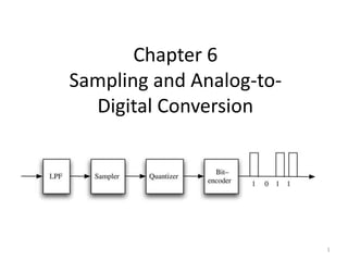
  • 1. 1 Chapter 6 Sampling and Analog-to- Digital Conversion
  • 2. 2 Content 1. Sampling Theorem 2. Pulse Code Modulation (PCM) 3. Digital Telephony: PCM in T1 Carrier Systems 4. Digital Multiplexing 5. Differential Pulse Code Modulation (DPCM) 6. Adaptive DPCM (ADPCM) 7. Delta Modulation
  • 3. 3 6.1 Sampling Theorem Significance Analog signals can be digitized through sampling and quantization. The sampling rate must be sufficiently large so that the analog signal can be reconstructed from the samples with sufficient accuracy. The sampling theorem, which is the basis for determining the proper sampling rate for a given signal, has a deep significance in signal processing and communication theory.
  • 4. 4 6.1 Sampling Theorem The theorem Any signal whose spectrum is band-limited to B Hz can be reconstructed exactly (without any error) from its samples taken uniformly at a rate fs >= 2B Hz (samples per second). In other words, the minimum sampling frequency is: fs = 2B Hz.
  • 5. 6.1 Sampling Theorem To prove the sampling theorem, consider a signal g(t) (Fig. 6.1 a) whose spectrum is band- limited to B Hz (Fig. 6.1b). Sampling g(t) at a rate of fs Hz can be accomplished by multiplying g(t) by an impulse train δTs(t) (Fig. 6.1c), consisting of unit impulses repeating periodically every Ts seconds, where Ts = 1/ fs.
  • 6. 6 6.1 Sampling Theorem 1/Ts x * Figure 6.1 Sampled signal and its Fourier spectra. 1/Ts                      n t f jn s n s s Ts s e t g T nT t nT g t t g t g    2 1         n n t jn s Ts s e T t   1           n s s nf f G T f G 1
  • 7. 7 6.1 Sampling Theorem Since the impulse train Ts(t) is a periodic signal of period Ts , it can be expressed as a Fourier series. Its exponential Fourier series is given by:               n s s Ts nT t nT g t t g t g           n n t jn s Ts s e T t   1 s s s f T    2 2                 n t f jn s T s s e t g T t t g t g   2 1 Therefore Taking the Fourier Transform:           n s s nf f G T f G 1 (Example 2.5 on page 45 of the text book) (Example 3.5 on page 74 and Example 3.11 on page 86 of the text book )
  • 8. If we are to reconstruct g(t) from ḡ(t), we should be able to recover G( f ) from Ḡ ( f ) using a LPF. This is possible if there is no overlap between successive cycles of Ḡ ( f ). This requires fs > 2B. Since the sampling interval is Ts=1/fs this implies Therefore, 1 2 S T B  The minimum sampling rate fs > 2B samples/second required to recover g(t) from its samples ḡ(t) is called the Nyquist rate for g(t), and the corresponding sampling interval Ts=1/(2B) seconds is called the Nyquist Interval for g(t). 6.1 Sampling Theorem
  • 9. 9 Signal Reconstruction: The Interpolation Formula           B f T f H s 2 The process of reconstructing a continuous-time signal g(t) from its samples is also known as interpolation. A signal g(t) band- limited to B Hz can be reconstructed (interpolated) exactly from its samples. This is done by passing the sampled signal through an ideal low-pass filter of bandwidth B Hz and gain Ts to recover the component (1/Ts)g(t) from the sampled signal. Thus, the reconstruction (or interpolating) filter transfer function is     Bt BT t h s  2 sinc 2 
  • 10. 10 Signal Reconstruction: The Interpolation Formula Assuming the Nyquist sampling rate, that is: 2B = fs = 1/Ts we obtain h(t) = sinc(2πBt)           B f T f H s 2     Bt BT t h s  2 sinc 2  h(t) = sinc(2πBt)
  • 11. 11 Signal Reconstruction: The Interpolation Formula The kth sample of the input ͞g(t) is the impulse g(nTs)δ(t- nTs); the filter output of this impulse is g(nTs)h(t-nTs). Hence the filter output ͞g(t), which is g(t), can now be expressed as a sum,                    n Bt nT g nT t B nT g nT t h nT g t g n s s n s s n s          2 sinc 2 sinc
  • 12. 12 Signal Reconstruction: The Interpolation Formula The above equation is the interpolation formula, which yields values of g(t) between samples as a weighted sum of all the sample values.         n Bt nT g t g n s    2 sinc
  • 13. 13 Practical Sampling Practical Sampling In proving the sampling theorem, we assumed ideal samples obtained by multiplying a signal g(t) by an impulse train which is physically nonexistent. In practice, we multiply a signal g(t) by a train of pulses of finite width, shown in the next figure. We wonder whether it is possible to recover or reconstruct g(t) from the sampled signal. Surprisingly, the answer is positive, provided that the sampling rate is not below the Nyquist rate. The signal g(t) can be recovered by low-pass filtering the sampled signal as if it were sampled by impulse train.
  • 14. 14 Practical Sampling The envelope is FT of a pulse x *
  • 15. Practical Sampling                                              n t f jn s n s n s n s s e T t p t g nT t t p t g nT t t p t g nT t p t g t g    2 1 * * * ~                                       n s s s n s s s n s s nf f G nf P T nf f nf P T f G nf f T f P f G f G 1 1 ~   Fourier Transform (spectrum) of the sampled signal is: Therefore g(t) can by reconstructed using a low pass filter (LPF) of B < Bandwidth < fs - B
  • 16. 16 Practical Sampling                 t g t p nT t nT g t p nT t p nT g t g n s s n s s * * ~         Therefore             n s s nf f G T f P f G 1 ~ Nevertheless in practical scenarios scaling factor for amplitude of each pulse can be considered a constant value over the pulse duration. In this case sampled signal Figure 6.5 Practical signal reconstruction.
  • 17. 17 Practical Sampling The equalizer must remove all the shifted replicas G( f - n fs) for n > 0 The sampling pulse can be approximated to rectangular pulses:              B f T B f f f P f E s s 0              p p T T t t p 5 . 0     sin p j fT p p P f T c fT e     To recover g(t) a filter (called equalizer) is needed. Let E(f) is the frequency response of the equalizer such that                    n s s nf f G T f P f E f G f E f G 1 ~
  • 18. 18 Practical Sampling As a result E( f ) must be :                         B f f B f f B Flexible B f f P T f E s s s 0     B f e fT f T f E p fT j p s    | | sin    By choosing Tp small:   B f T T f E p s   | |
  • 19. 19 Maximum Information Rate A minimum of 2B independent pieces of information per second can be transmitted, error free, over a noiseless channel of bandwidth B Hz. This can be proved by the sampling theorem.
  • 20. 20 Some Applications of the Sampling Theorem Figure 6.11 Pulse-modulated signals. (a) The unmodulated signal. (b) The PAM signal. (c) The PWM (PDM) signal. (d) The PPM signal.
  • 21. 21 Some Applications of the Sampling Theorem Figure 6.12 Time division multiplexing of two signals.
  • 22. 22 6.2 Pulse Code Modulation PCM is the most used among the pulse modulation techniques. It is used to convert analog signal to digital one. After quantizing a sampled signal we obtain a L-level pulse train. This signal can be converted to “binary pulses” by assigning a binary code for each level. Thus the L-ary signal is converted to a binary signal where the 0 and 1 can be expressed as -1V and +1V. Figure 6.13 PCM system diagram.
  • 23. 23 Quantization Figure 6.14 Quantization of a sampled analog signal.
  • 26. 26 Pulse Code Modulation Example1: telephony systems Step1: the bandwidth is limited to 3400Hz (enough for intelligibility) with low pass filter. Step2: the resulting signal is sampled with fs = 8000Hz (> 6.8KHz). Step3: the samples are quantized to 256 levels = 28. Step4: the quantized levels are then coded with 8-bit binary code.  the telephone signal require a rate of 8000x 8 =64000 binary pulses per second (64kbps).
  • 27. 27 Pulse Code Modulation Example2: compact disc CD Step1: the bandwidth is limited to 15kHz, since it is a HIFI system. Step2: the resulting signal is sampled with fs = 44.1kHz (> 30kHz). Step3: the samples are quantized to 65,536 levels = 216. Step4: the quantized levels are then coded with 16-bit binary code.  the binary pulses are then recorded in the CD
  • 28. 28 2.2 Uniform Quantizing Figure 6.14 Quantization of a sampled analog signal.
  • 29. 29 2.2 Uniform Quantizing In digital communication, the detection error is usually much less than the quantizing error and can be ignored i.e., the detection error is ignored. For quantizing, we limit the amplitude of the message signal m(t) to the range (-mp, mp), as shown in Fig. 6.10. Note that mp is not necessarily the peak amplitude of m(t). The amplitudes of m(t) beyond ±mp are chopped off. Thus, mp is not a parameter of the signal m(t), but is a constant of the quantizer. The amplitude range (-mp, mp) is divided into L uniformly spaced intervals, each of width Δv = 2mp/L.
  • 30. (a) Quantizer characteristic of a uniform quantizer (b) Error signal v v v v v v v v v/2 v/2 v/2 v/2 v/2 v/2 v/2 v/2 Quantizer Input x Quantizer Output xq q x x mp v v v v v v v v v/2 Quantizer Input x Quantization Error q v/2 mp (a) (b) Quantizing Error (noise) Uniform Quantizer Δv = 2mp/L = x-xq
  • 31. Example: A signal m(t) with amplitude variations in the range -mp to mp is to be sent using PCM with a uniform quantizer. The quantization error should be less than or equal to 0.1 percent of the peak value mp. If the signal is band limited to 5 kHz, find the minimum bit rate required by this scheme. Ans: 105 bps
  • 32. 32 Quantizing Noise The mean square of the original signal is:   t m S 2 0  The mean square of the quantization error is: 2 2 2 0 3 12 L m v N p    Where L, number of the quantizer levels and mp is the highest quantizer level. (a constant of the quantizer) The SNR, signal to noise ratio is given by:   2 2 2 0 0 3 p m t m L N S SNR   Δv = 2mp/L
  • 33. 33 2.3 Non-uniform Quantizing Normally we prefer a constant SNR. Unfortunately it is not the case. The SNR is directly related to the mean power of the signal varying from one talker to another. They also vary with the path length. This is due to the fact that the quantizer step is constant v = 2mp / L. The quantizing error is directly proportional to the step size. How to maintain a constant SNR for different signals?
  • 34. 34 Non-uniform Quantizing Solution  Taking smaller steps for small signals and larger steps for large signals.  nonuniform quantizing.  Same result can be obtained by signal compression followed by quantization with uniform-step quantizer e.g. logarithmic compression Compression function
  • 35. 35 Non-uniform Quantizing smaller quantization noise for small signal. SNR independent from the signal power for large dynamic range  disadvantage: more noise in strong signals.
  • 36. 36 Non-uniform Quantizing              p m m y   1 ln 1 ln 1 1 0   p m m                                    1 1 1 ln ln 1 1 1 0 ln ln 1 1 p p p p m m A m Am A A m m m m A y Compression laws: law (in North America and Japan) Alaw (In Europe and the rest of the world)
  • 38. 38 Non-uniform Quantizing The coefficients  or A define the degree of compression.  For 128-level (7 bits) encoding,  = 100 is used leading to a dynamic range of 40dB.  For 256-level (8 bits) encoding,  = 255 is used leading to a dynamic range of 40dB.  For 256-level (8 bits) encoding, A = 87.6 is used leading to a comparable results.
  • 39. • A number of companies manufacture CODEC chips with various specifications and in various configurations. Some of these companies are: Motorola (USA), National semiconductors (USA), OKI (Japan). • These ICs include the anti-aliasing bandpass filter (300 Hz to 3.4 kHz), receiver lowpass filter, pin selectable A-law / μ -law option. Listed below are some of the chip numbers manufactured by these companies. Motorola: MC145500 to MC145505 National: TP3070, TP3071 and TP3070-X OKI: MSM7578H / 7578V / 7579 Details about these ICs can be downloaded from their respective websites.
  • 40. 40 Non-uniform Quantizing At the receiver end an expander must be used to restore the original signal. The compressor and the expander are together called the compander. In  -law compander the SNR is found to be:       t m m for L N S p 2 2 2 2 2 0 0 ~ 1 ln 3     
  • 42. 42 Non-uniform Quantizing Compander Based on logarithmic diode characteristics.           s I I q KT V 1 ln Encoder and Decoder  Sampling, quantization and encoding are performed using the Analog to Digital Converter  Digital to Analog Converter can be used for decoding.
  • 43. 43 Comments on Logarithmic Units (Decibel)  Voltage: V = x Volt  VdB = 20log10(x).  Ratio between voltages: A = V1/V2  AdB = 20log10(A).  Power: P = y Watt  PdB = 10log10(y). P = y mWatt  PdBm = 10log10(y). PdBm = PdB + 30  Ratio between Powers: G = P1/P2 =  GdB = 10log10(G).
  • 45. 45 2.3 Transmission Bandwidth and the Output SNR For a binary PCM, we assign a distinct group of n binary digits (bits) to each of the L quantization levels. Because a sequence of n binary digits can be arranged in 2n distinct patterns, L = 2n or n = log2 L (6.37) Each quantized sample is, thus, encoded into n bits. Because a signal m(t) band-limited to B Hz requires a minimum of 2B samples per second, we require a total of 2nB bits per second (bps), that is, 2nB pieces of information per second. Because a unit bandwidth (1 Hz) can transmit a maximum of two pieces of information per second, we require a minimum channel of bandwidth BT Hz, given by BT = nB Hz (6.38)
  • 46. 46 Pulse Code Modulation (6.37) (6.40) (6.39) (6.41) (6.34) (6.36) (6.34) (6.36) (6.38) (6.39) (6.40)
  • 48. 48 Digital Telephony: PCM in T1 Carrier Systems 24 analog channels sampled (PAM)  time multiplexed (TDM)  quantized (256-level)  encoded (8-bit PCM)  sent to transmission medium with repeaters at each 6000ft. At the receiver, the signal is decoded (converted to samples)  the samples are demultiplexed to 24 channels  the signal of each channel is filtered (LPF) to restore the desired audio signal. The 1.544MB/s signal of the T1 is called Digital Signal Level 1 (DS1), used to build higher DS, (DS2, DS3, DS4). It is used in North America and Japan. Now the standard is the 30-channel 2.048MB/s PCM system used around the world, except North America and Japan who stayed using the T1. Interfaces are developed for international communication.
  • 49. 49 3. Digital Telephony: PCM in T1 Carrier Systems
  • 50. 50 Digital Telephony: PCM in T1 Carrier Systems Synchronization and signaling Synchronization Frame: 192 bits = 8 bits x 24 channel (1 sample for each channel). Sample rate (1 ch.): 8000 Samples/s  each frame takes 125s. At the receiver end it is difficult to catch the beginning of each frame. To solve the problem and separate the information bit correctly, a framing bit is added to the frame  the total number of bits in a frame is 193. The framing bits are used in a way that they form a special pattern unlikely to be used in voice speech. At the receiver end, the receiver examines the bits until it gets the pattern  it catches the beginning of the frame. This is called synchronization. It takes 0.6 to 6 ms.
  • 51. 51 Digital Telephony: PCM in T1 Carrier Systems
  • 52. 52 Digital Telephony: PCM in T1 Carrier Systems Signaling It consists of sending information relative to the dialing pulses and the on-hook/off-hook signals. These information are useful for telephone switching systems. Instead of allocating time slots for this information we take the LSB of every sixth sample of a transmitted signal. This is called encoding and the signaling channel so derived is called robbed- bit-signaling.  this result in a small acceptable deterioration in the SNR of the signal. The rate of the signaling bit for each channel is 8000 / 6 = 1333 b/s 5 7 6
  • 53. 53 Digital Telephony: PCM in T1 Carrier Systems Question: How can we detect frames that contain the signaling bits at the receiver end? Answer: superframe technique: the pattern used to detect the beginning of each frame is also used to detect the beginning of each superframe (12 frames)  2 signaling bits per channel can be detected in each superframe [equivalent to 4-state signaling (00, 01, 10, 11)].
  • 54. Differential Pulse Code Modulation (DPCM)  DPCM can be treated as a variation of PCM; it also involves the three basic steps of PCM, namely, sampling, quantization and coding.  In DPCM, what is quantized is the difference between the actual sample and its predicted value.  DPCM exploits the correlation between adjacent samples of the signal, to improve A/D conversion efficiency.  Quite a few real world signals such as speech signals, biomedical signals (ECG, EEG, etc.), telemetry signals (temperature inside a space craft, atmospheric pressure, etc.) do exhibit sample-to-sample correlation .
  • 55. Differential Pulse Code Modulation (DPCM) Correlation  samples m[k] and m[k+1] (or m[k-1] and m[k]) do not differ significantly. Given a set of previous N samples m[k-1], m[k-2],…,m[k-N] m[k] can be predicted with a small error. Let denote the predicted value of m[k]. Then the error is: Instead of transmitting m[k], d[k] is transmitted. Peak of d[k] is significantly smaller than the peak of m[k]. Therefore the parameter mp of the quantizer is reduced.   m̂ k       ˆ d k m k m k  
  • 56. Differential Pulse Code Modulation (DPCM) For a given L, the quantization interval Δv = 2mp/L is reduced compared to PCM. Can be used in two ways. (1) the quantization noise is reduced  is increased. (2) On the other hand for a given SNR, L can be reduced compared to PCM number of bits/sample, n=log2 L can be reduced. Decoding At the receiver the estimate is found using the past samples and d[k] is added to calculate m[k]. 2 2 2 0 3 12 L m v N p      2 2 0 2 0 3 p m t S SNR L N m     m̂ k
  • 57. Deficiency: At the receiver, instead of the past samples m[k-1], m[k-2],… we only have the quantized version of the sequence mq[k-1], mq[k-2],… and the quantized version of the difference dq[k]. Therefore cannot be predicted. Only the estimate of the quantized sample can be predicted Solution: determine at the transmitter from mq[k-1], mq[k-2],… and find . Then transmit the quantized version  dq[k]=d[k]+q[k] where q[k] is the quantization error.       ˆq d k m k m k     m̂ k   ˆq m k   ˆq m k
  • 58.                 ˆ q q q q m k m k d k m k d k d k m k q k        Predictor input is indeed mq[k]. Receiver can find the quantized version of m[k].   q m k   ˆq m k (a) DPCM transmitter (b) DPCM receiver m[k] d[k] dq[k] dq[k]   ˆq m k   q m k   q m k Similar to receiver   ˆq m k   q m k       ˆq d k m k m k   dq[k]=d[k]+q[k]
  • 59. Delta Modulation (DM)  Delta modulation is a predictive waveform coding technique and can be considered as a special case of DPCM. Uses the simplest possible quantizer, namely a two level (one bit) quantizer. The price paid for achieving the simplicity of the quantizer is the increased sampling rate (much higher than the Nyquist rate). Over-sampling is used in order to increase the adjacent sample correlation. like in DPCM, acts on the difference (prediction error) signals.
  • 60. Waveforms illustrative of LDM operation Linear (or non-adaptive) Delta Modulator (LDM)
  • 61. Discrete-time LDM system (a) Transmitter (b) Receiver Delta modulation is a special case of DPCM. m[k] d[k] dq[k]   1 q m k    q m k   q m k   1 q m k 
  • 62.
  • 63. 63 Advantages of Digital Communication (over analog communication) 1. More immunity to noise and distortion. 2. Possibility of regeneration. (repeaters)  avoid accumulation of signal distortion along the transmission path. (which is difficult to avoid in analog Communication systems) 3. Digital hardware implementation is more flexible.  use of DSP, micro-processors, mini-processor, VLSI etc. 4. Signal can be coded for protection against error and piracy. 5. More flexibility in exchanging SNR and bandwidth.
  • 64. Advantages of Digital Communication (over analog communication) 5. Easier and more efficient in multiplexing several signals. 6. Easier in storage and search. 7. Reproduction of digital signal is extremely reliable. Analog signal is more and more deteriorated with successive reproduction. 8. Cost/performance criteria will cause the digital communication and data storage to dominate over the analog systems. (due to the increasing performance of digital circuits and its decreasing cost)