Downloaded 18 times

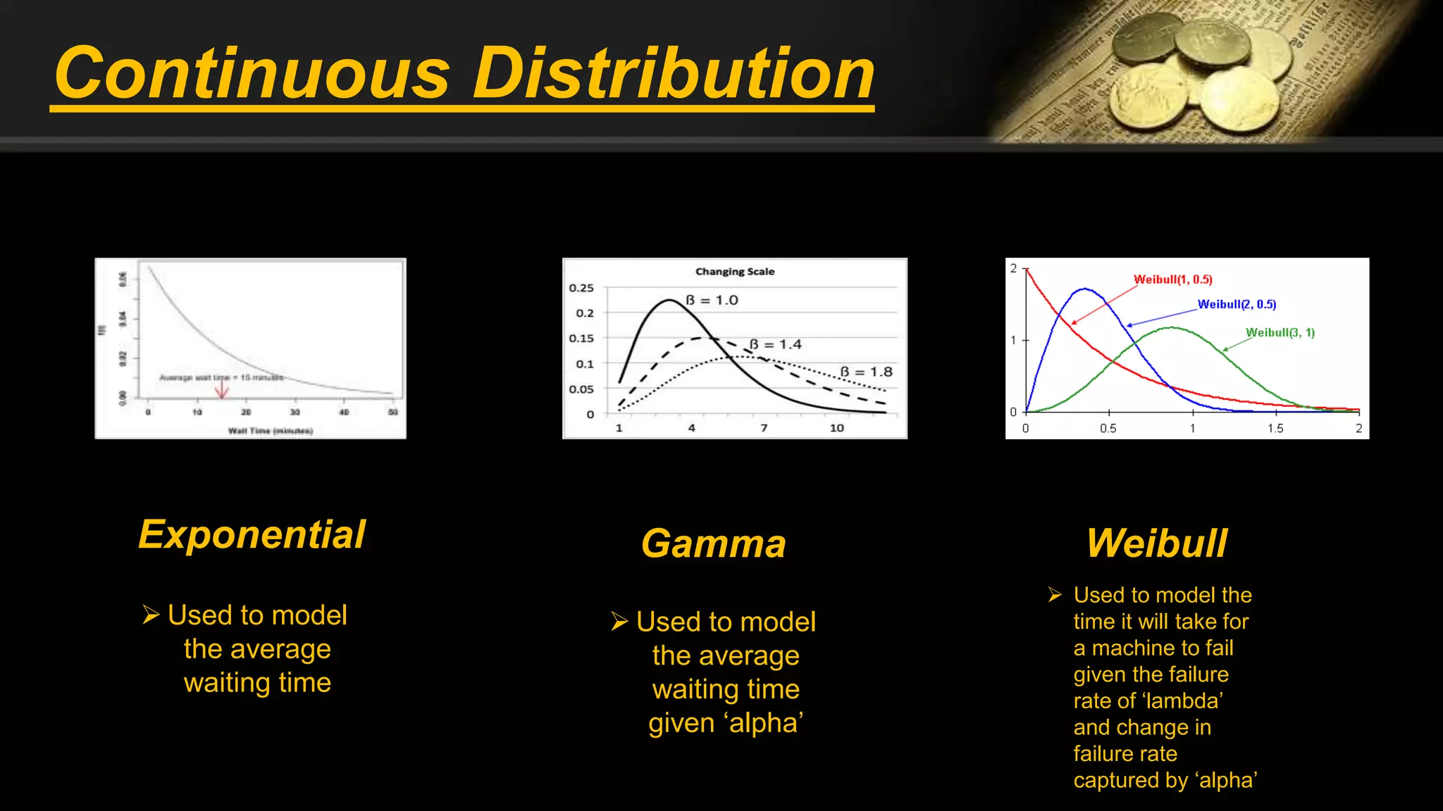
![Exponential Distribution
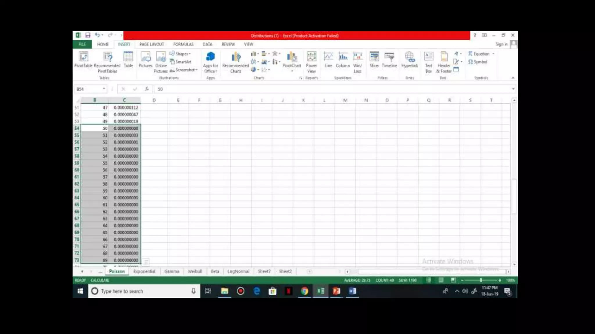
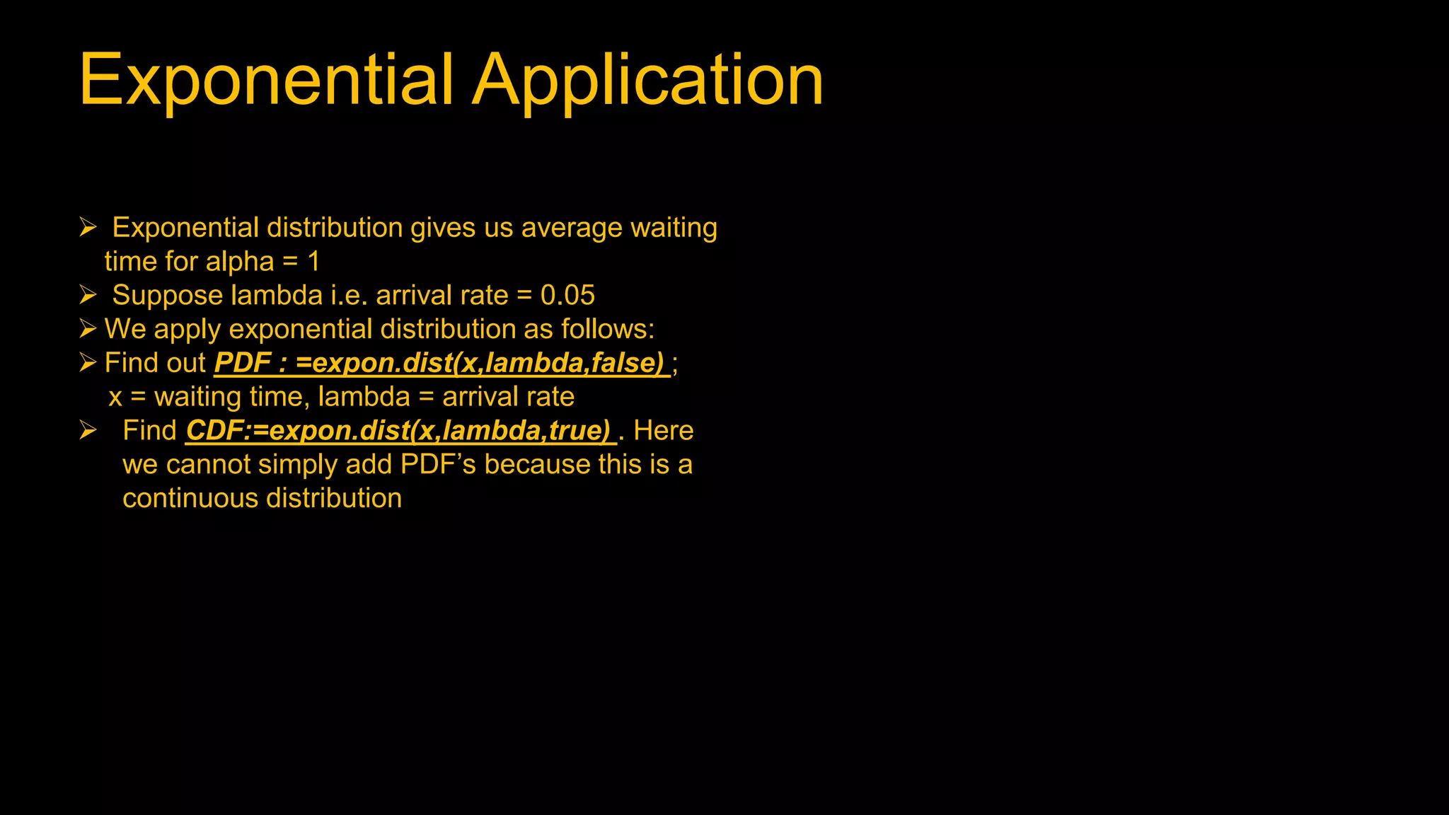
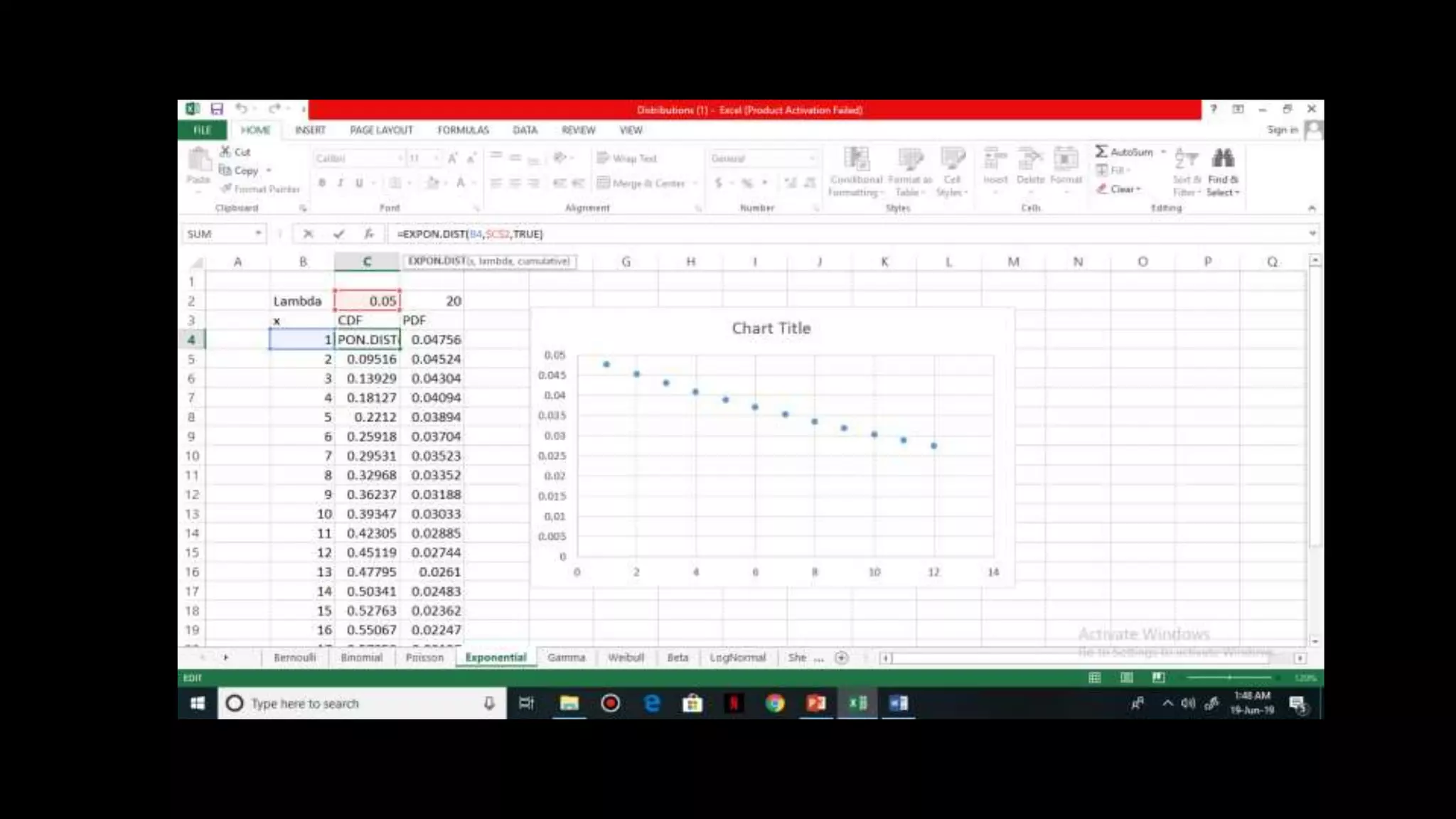
It is a continuous distribution and is used to model
average waiting time
Parameter of Exponential distribution = lambda
Mean = 1 / lambda
Variance = 1 / lambda^2
CDF , F(X) = 1 – e^ [(-lambda) * X]
PDF, f (X) = lambda * e^ [(-lambda) * X]
Survival probability = e^ [(-lambda) * X]](https://image.slidesharecdn.com/distributionppt-190701102145/75/Probability-Distribution-Modelling-19-2048.jpg)
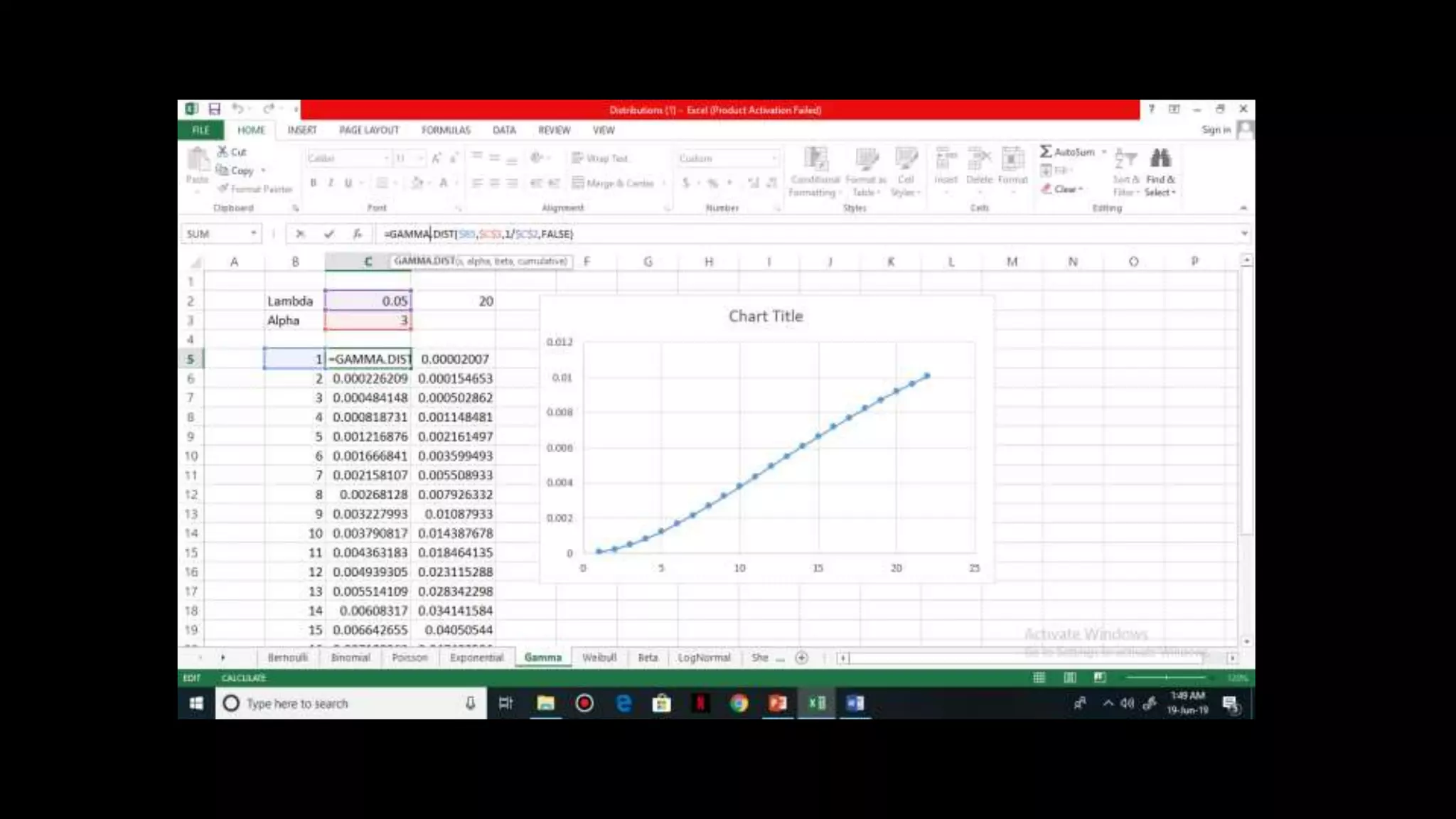
![Gamma Distribution
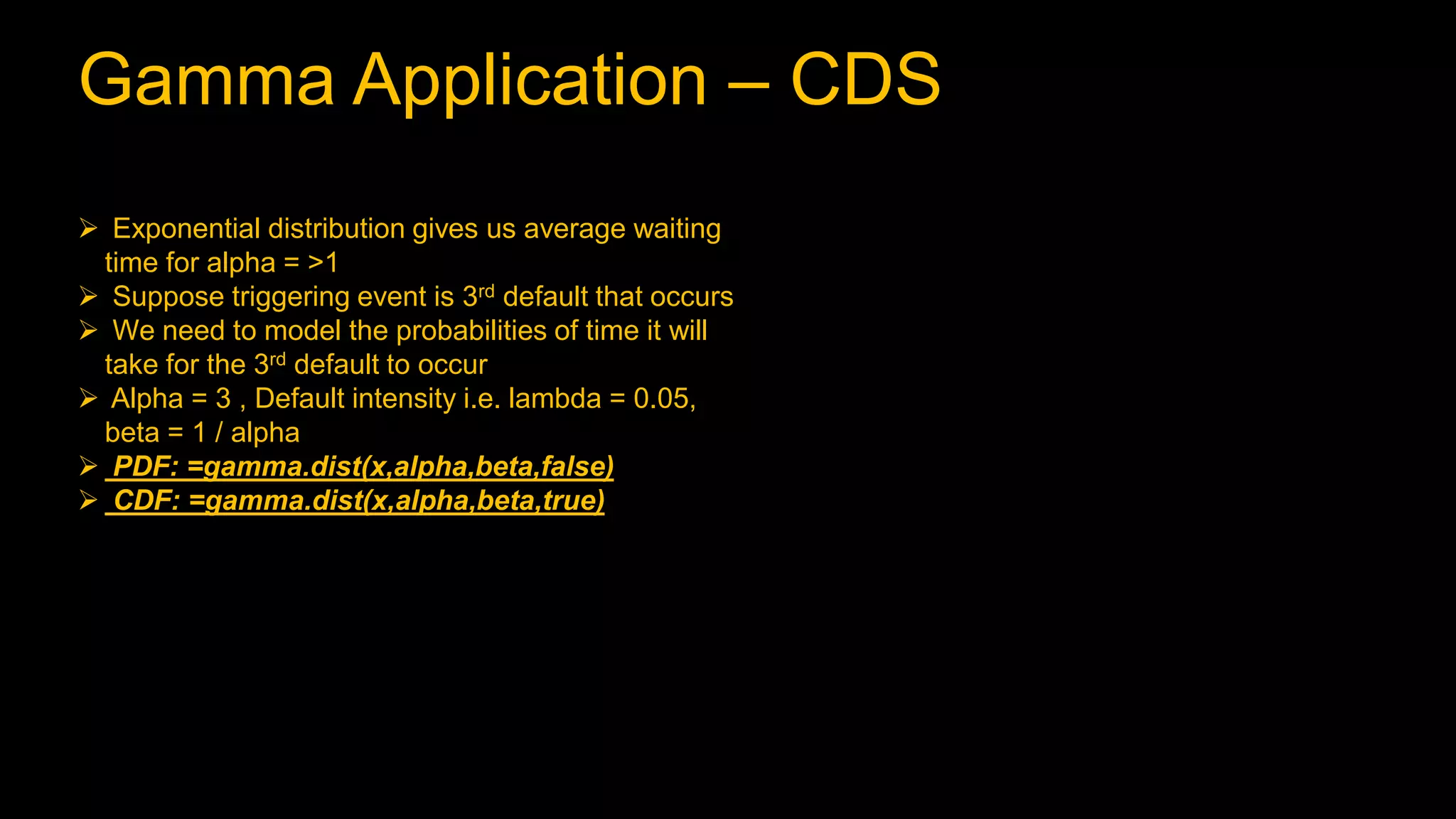
It is a continuous distribution and is used to model
average waiting time for alpha = >1
Parameter of Gamma distribution = alpha & lambda
Mean = alpha / lambda
Variance = alpha / lambda^2
CDF , F(X) = 1 – e^ [(-lambda) * X]
PDF, f (X) = lambda * e^ [(-lambda) * X]
Practically used in Credit Default Swaps to model the
time it will take for triggering event to occur](https://image.slidesharecdn.com/distributionppt-190701102145/75/Probability-Distribution-Modelling-22-2048.jpg)
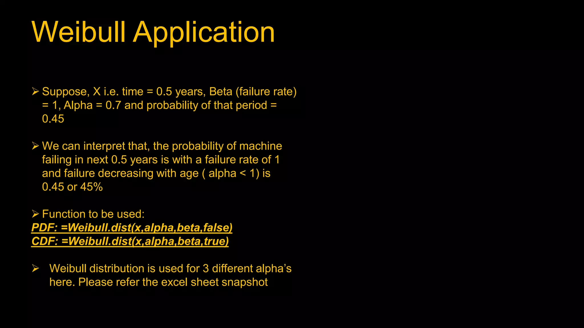
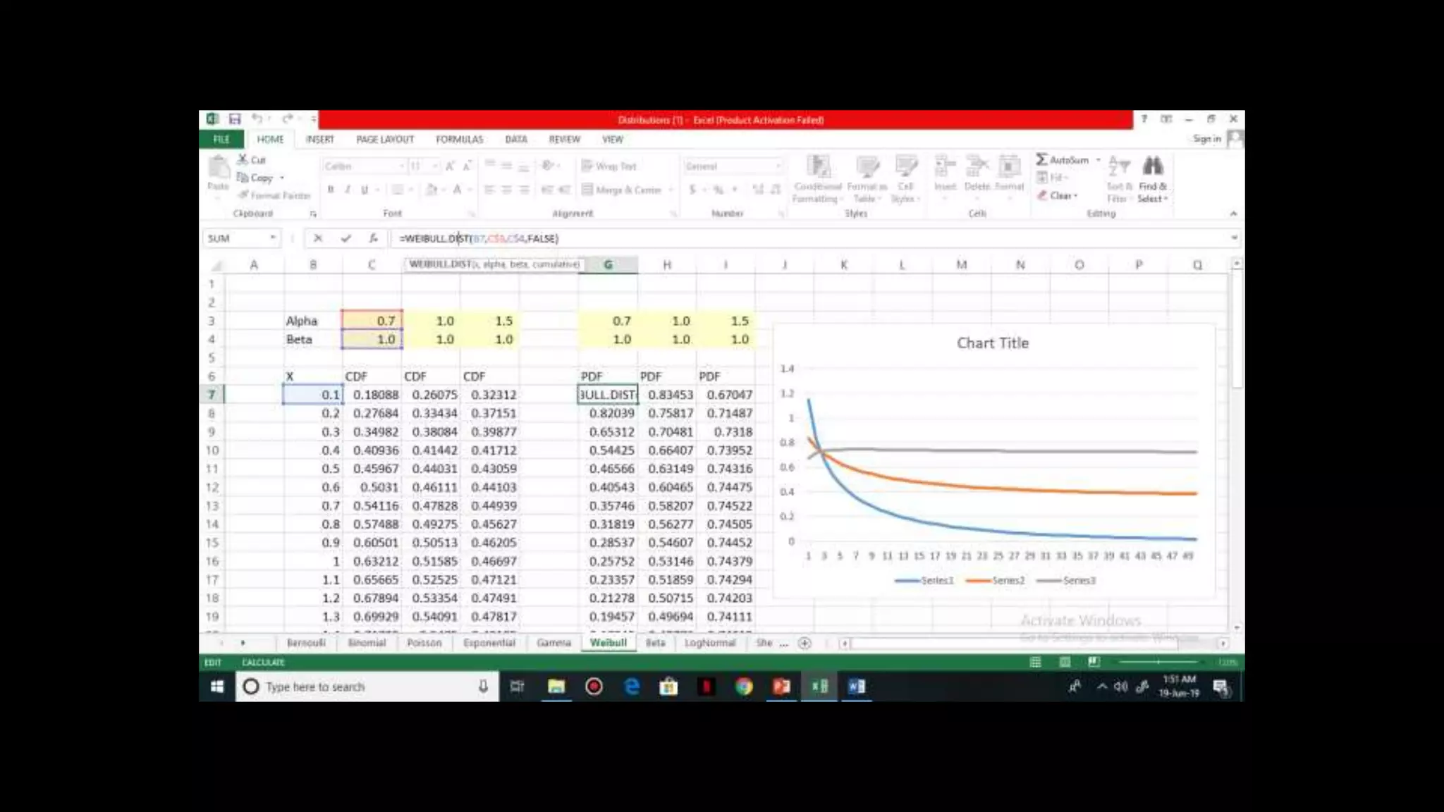
![Weibull Distribution
Used to model the time it will take for the machine to
fail given the failure rate of lambda
Change in failure rate (Constant/Increase/Decrease)
is captured by Alpha
If failure rate is constant, alpha = 0 exponential
If failure rate increases, alpha>1 Ageing problem
If failure rate decreases, alpha<1 Teething problem
CDF, F(X) = 1 – e^{[(-lambda) * x]^alpha}
Beta = 1 / alpha](https://image.slidesharecdn.com/distributionppt-190701102145/75/Probability-Distribution-Modelling-25-2048.jpg)
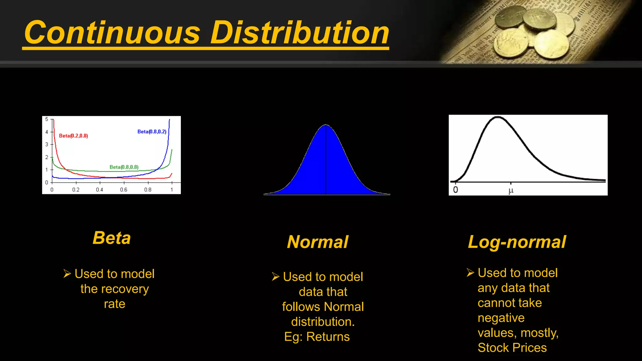
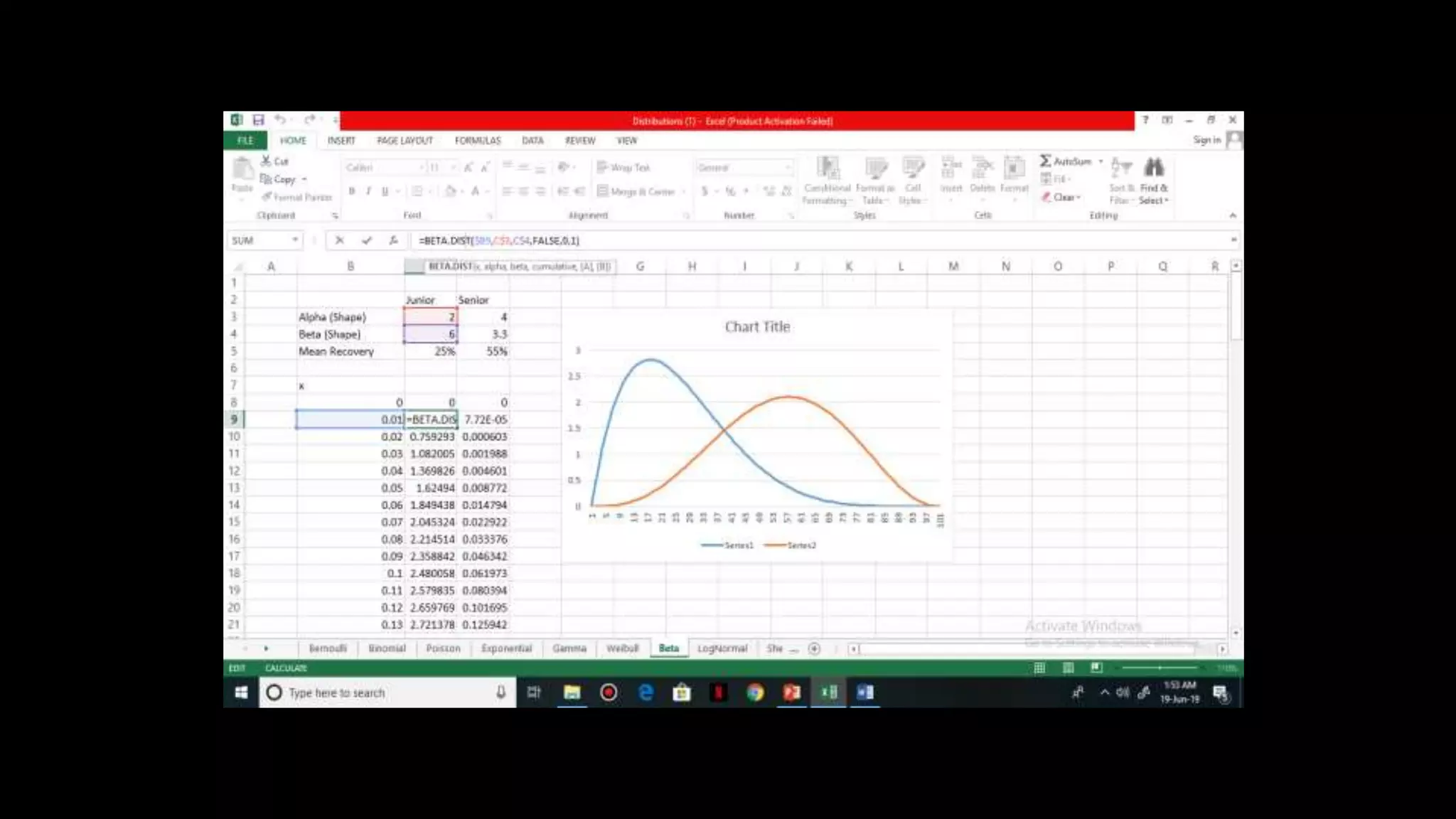
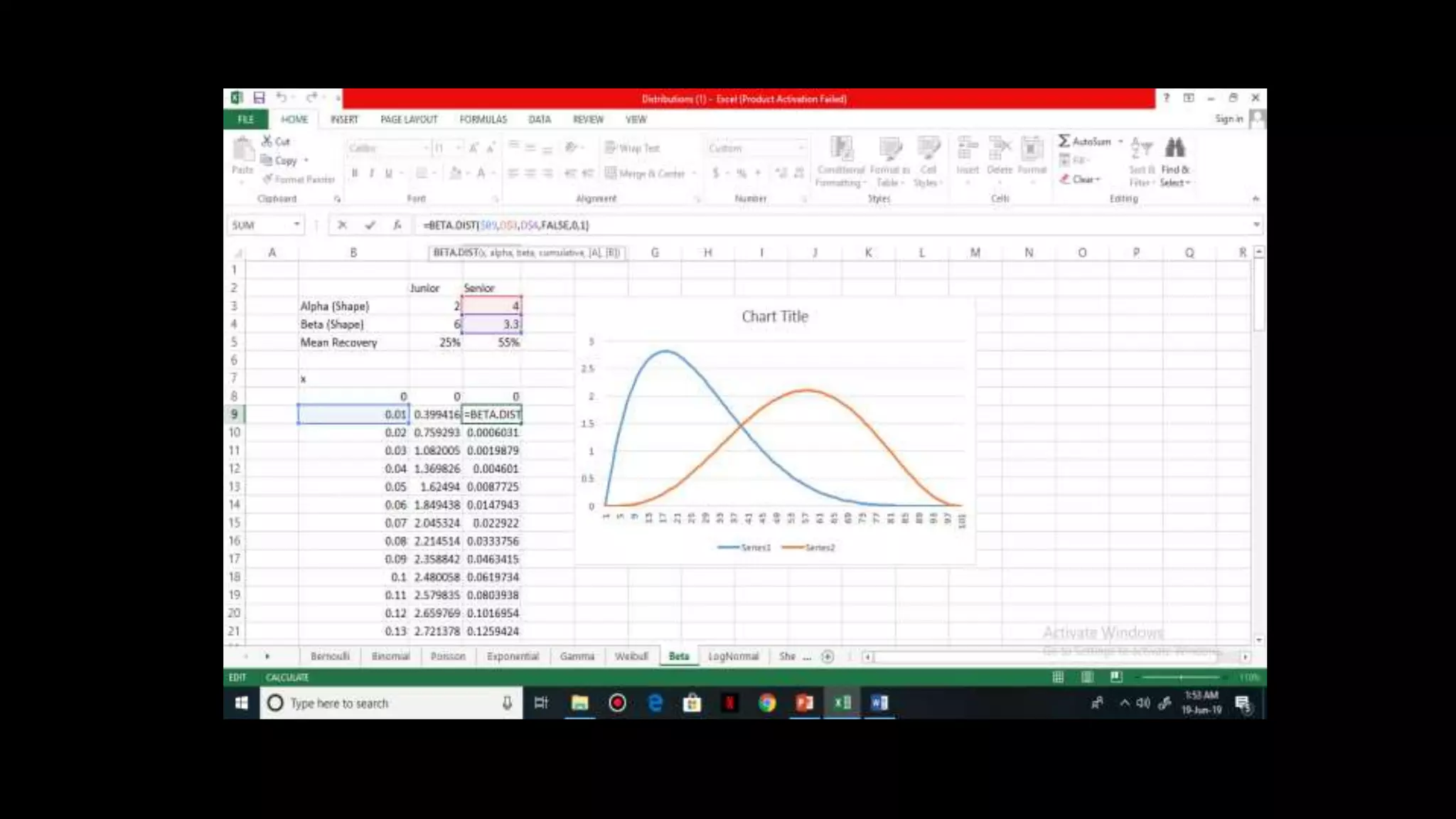
![Beta Distribution
It is a continuous distribution and is used to model
recovery rate
Parameters of beta distribution = alpha & beta
Mean = alpha / alpha + beta
CDF, F(X) = 1 – e^{[(-lambda) * x]^alpha}
Beta = 1 / alpha](https://image.slidesharecdn.com/distributionppt-190701102145/75/Probability-Distribution-Modelling-28-2048.jpg)


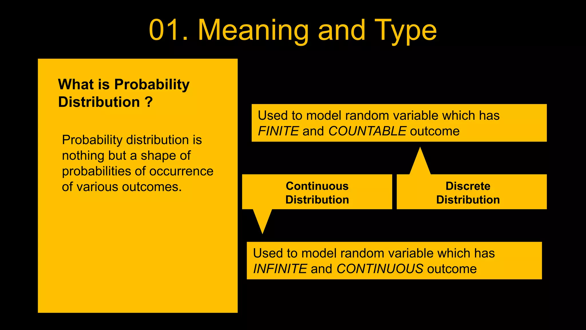
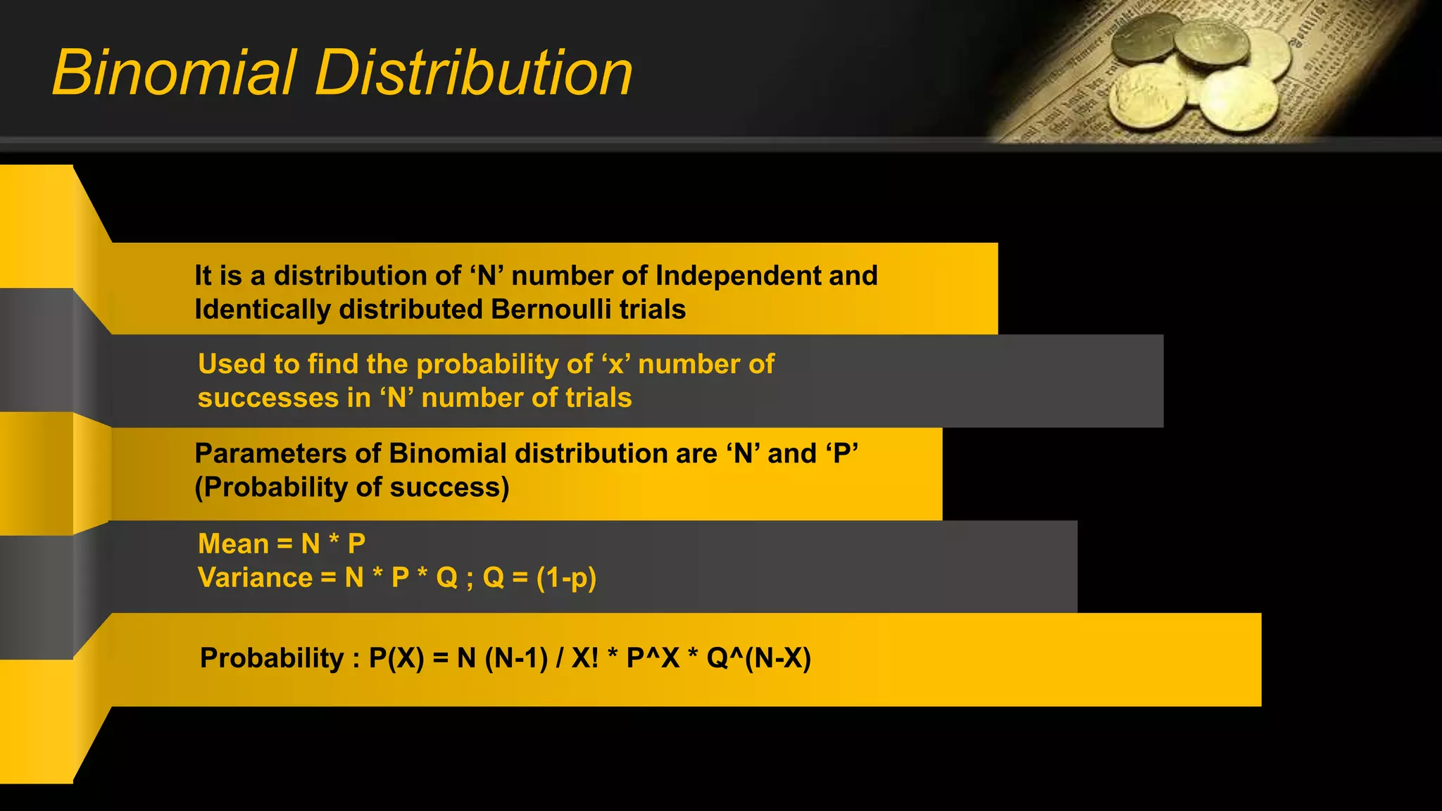
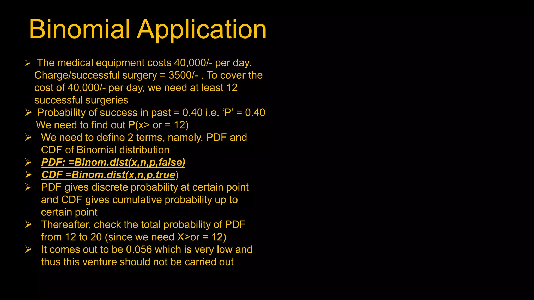
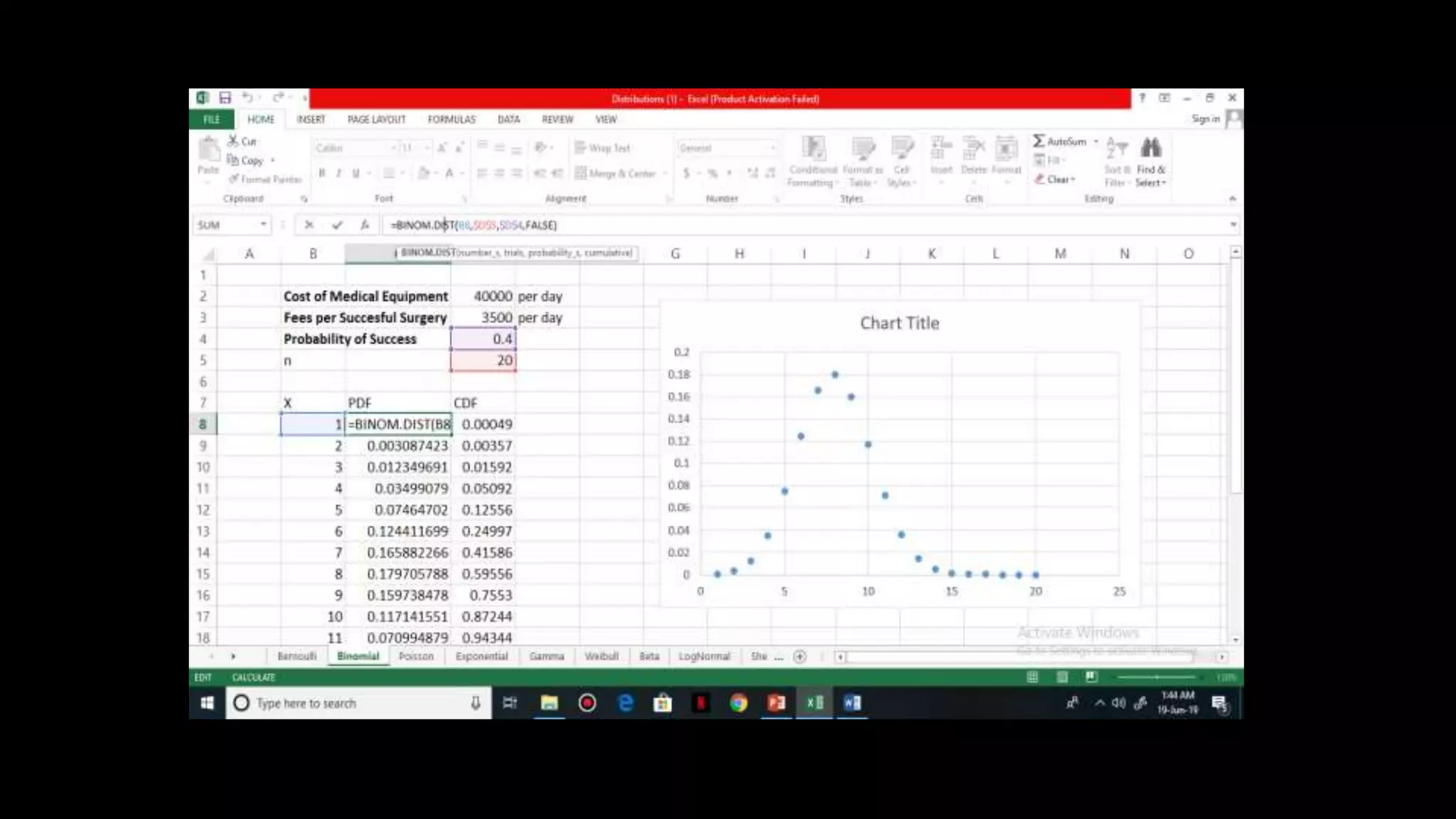
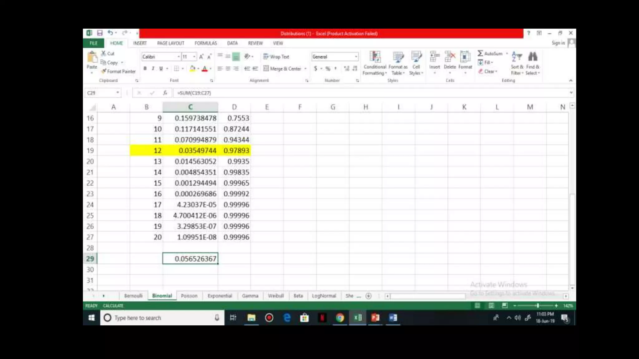
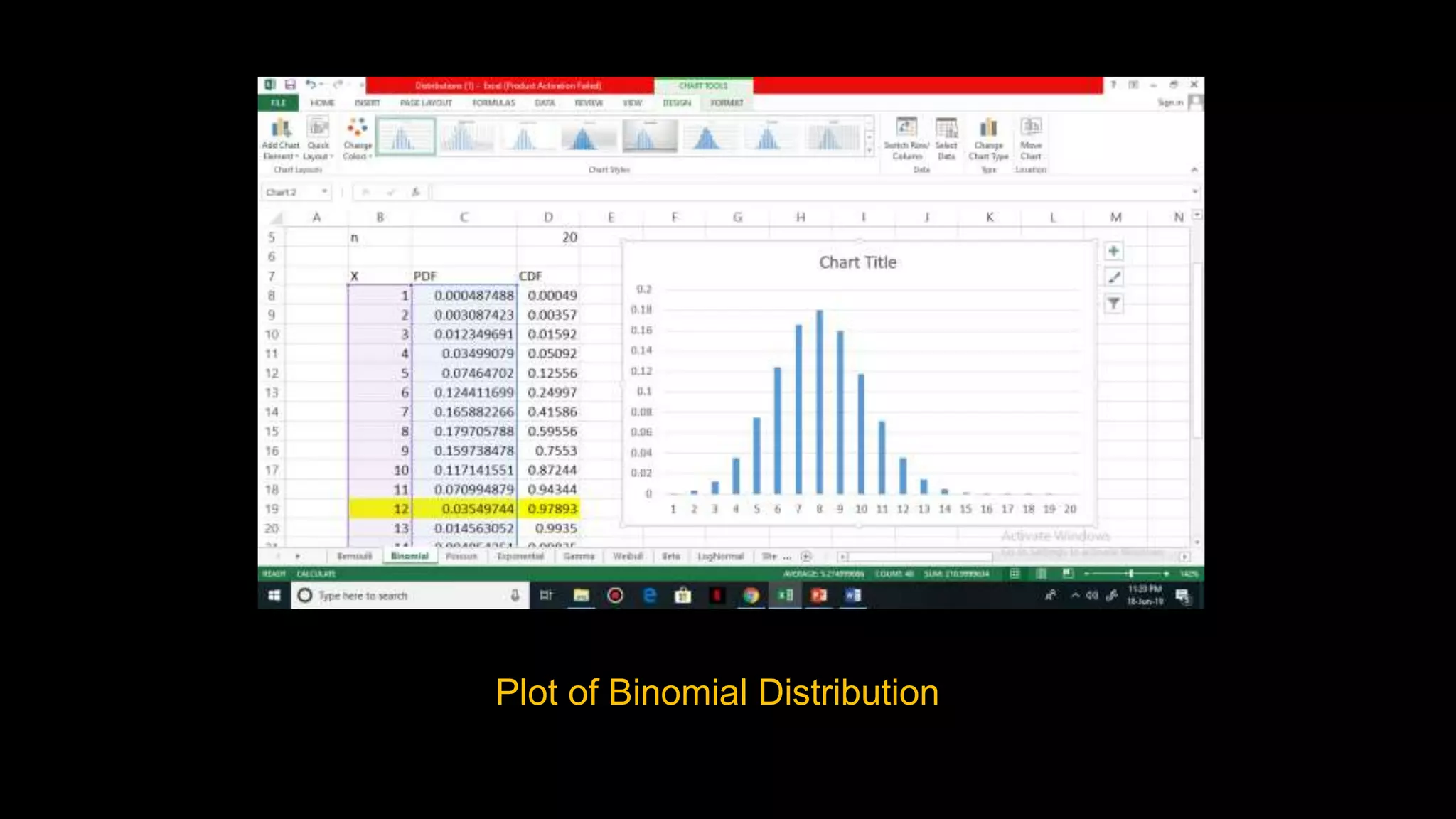
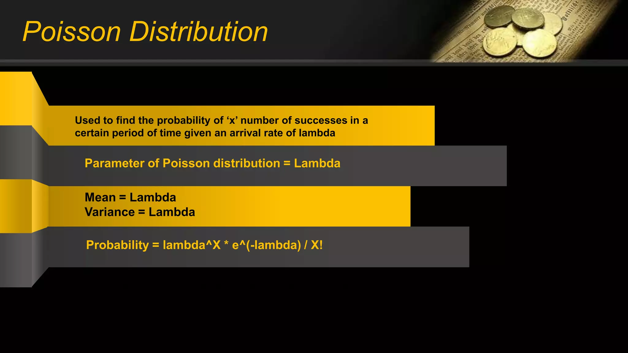
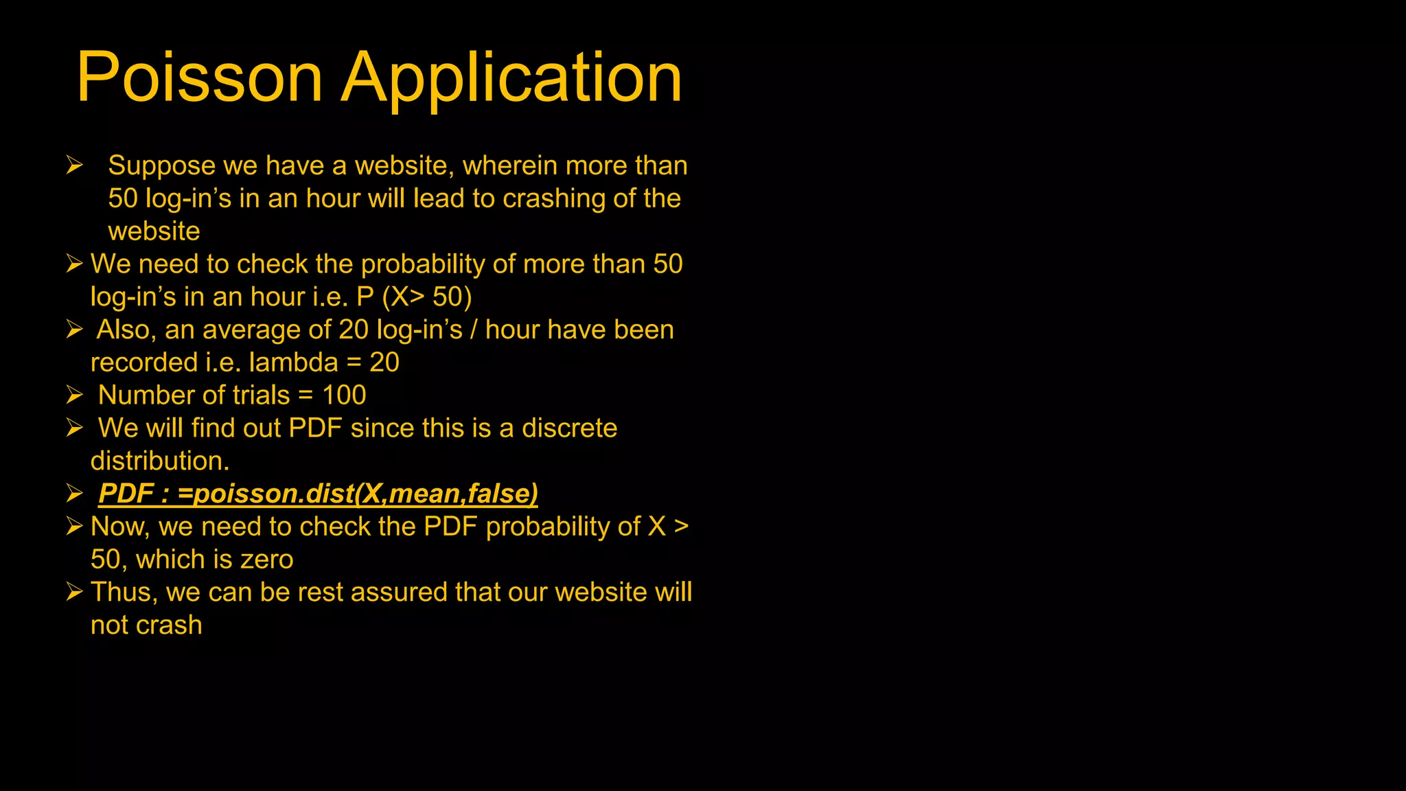
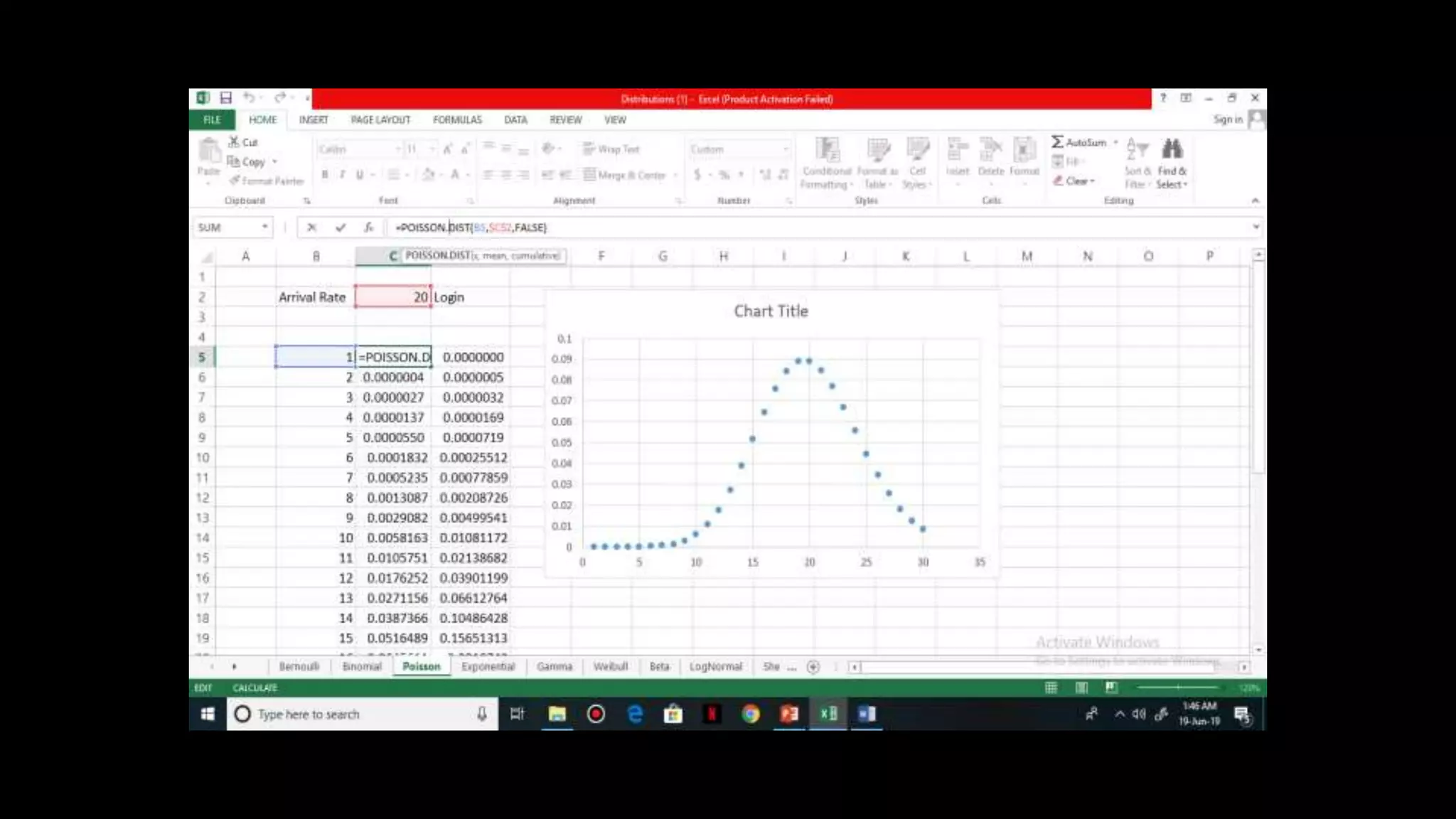
This document provides an overview of various probability distributions including discrete and continuous distributions. It defines key probability distributions such as binomial, Poisson, exponential, gamma, Weibull, beta, and log-normal distributions. Examples are given for how each distribution can be used to model different types of random variables and calculate probabilities. Applications of several distributions are demonstrated through examples in finance, healthcare, and engineering to show how the distributions can be used to model real-world scenarios.


![[DSC Europe 25] Uros Pesic - The Reality of AI in Marketing.pdf](https://cdn.slidesharecdn.com/ss_thumbnails/rtkodnmtycovsllvzsyn-9-251215095918-b0c6bfe3-thumbnail.jpg?width=640&height=640&fit=bounds)


![[DSC Europe 25] Ivan Peric - Intelligence Swarm Logic and Techno-Functional M...](https://cdn.slidesharecdn.com/ss_thumbnails/7my7c97fsduiccadgavw-2-251212103249-5a03f7c6-thumbnail.jpg?width=640&height=640&fit=bounds)
![[DSC Europe 25] Kaja Kandare - LLM as a judge.pptx](https://cdn.slidesharecdn.com/ss_thumbnails/arxyccaxsdsd1ba99wjw-7-251212104007-2b4e3f64-thumbnail.jpg?width=640&height=640&fit=bounds)

![[DSC Europe 25] Hans Kleinsman - The Compliance Gearbox: How Tax Tech Mediate...](https://cdn.slidesharecdn.com/ss_thumbnails/dxdytie1toel0hr90bjs-2-251212103250-174fdbe7-thumbnail.jpg?width=640&height=640&fit=bounds)

![[DSC Europe 25] Branko Dzakula - From Defense to Attack: How AI Redefines Cyb...](https://cdn.slidesharecdn.com/ss_thumbnails/80bdzdxpr3ky2g0qvyk9-8-251211083048-ce5fc1ee-thumbnail.jpg?width=640&height=640&fit=bounds)
![[DSC Europe 25] Milan Sekuloski - Data, Defence, and Development: Cybersecuri...](https://cdn.slidesharecdn.com/ss_thumbnails/dfrkwwx4qly6atqpbl4z-4-251209104645-c3d4b0ca-thumbnail.jpg?width=640&height=640&fit=bounds)
![[DSC Europe 25] Marko Krstic - Understanding the AI Threat Landscape - Risks,...](https://cdn.slidesharecdn.com/ss_thumbnails/tiyim1ins5jvbrvzpzla-2-251209104645-c69d3553-thumbnail.jpg?width=640&height=640&fit=bounds)
