Download to read offline


![Activity 4. 1
X is a normally normally distributed variable with mean μ = 30 and standard deviation σ = 4. Find
a) P(x < 40)
b) P(x > 21)
c) P(30 < x < 35)
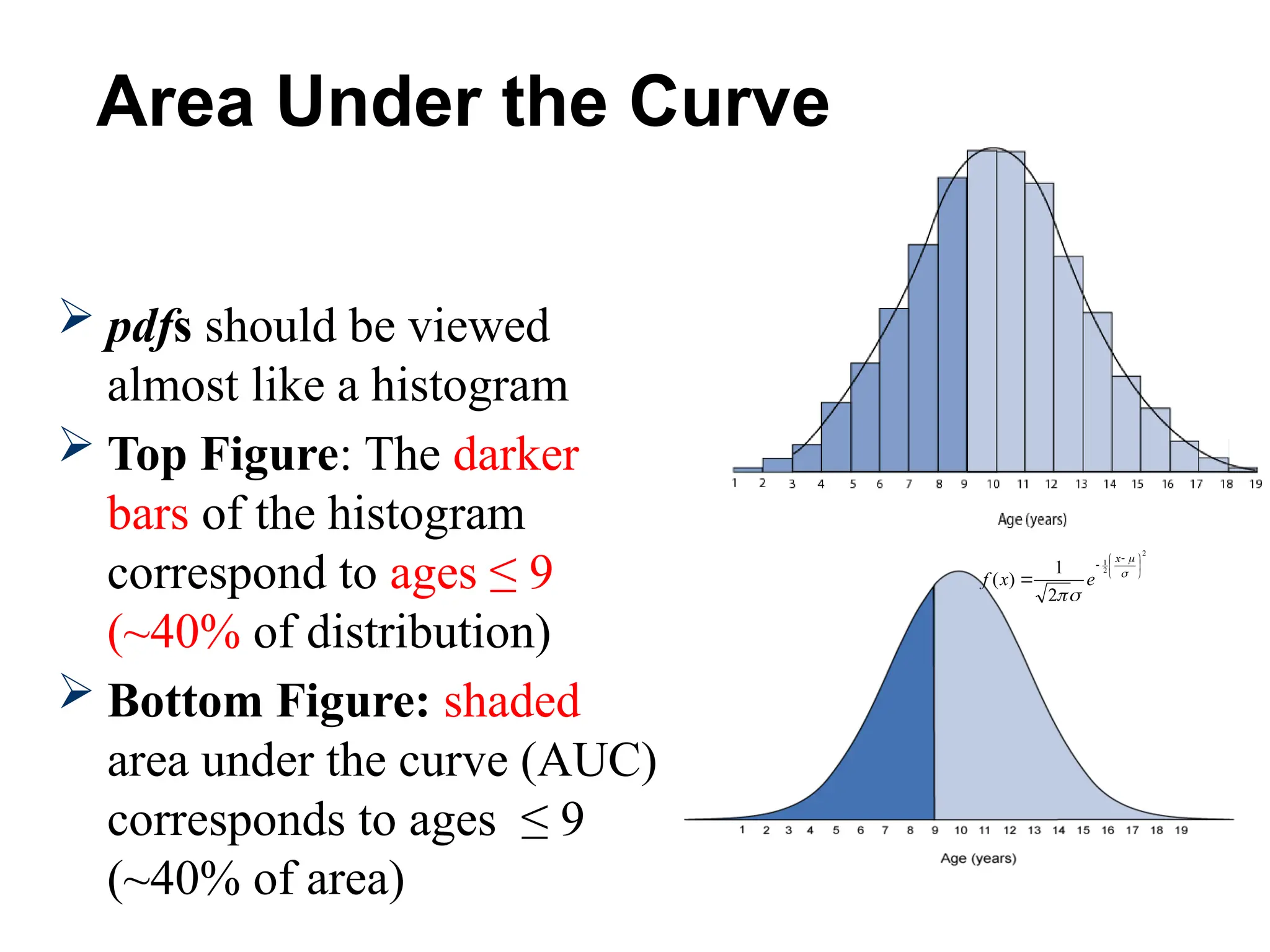
● Note: What is meant here by area is the area under the standard normal curve.
● Solution
a) For x = 40, the z-value z = (40 - 30) / 4 = 2.5
Hence P(x < 40) = P(z < 2.5) = [area to the left of 2.5] = 0.9938
b) For x = 21, z = (21 - 30) / 4 = -2.25
●
Hence P(x > 21) = P(z > -2.25) = [total area] - [area to the left of -2.25]
= 1 - 0.0122 = 0.9878
c) For x = 30 , z = (30 - 30) / 4 = 0 and for x = 35, z = (35 - 30) / 4 = 1.25
Hence P(30 < x < 35) = P(0 < z < 1.25) = [area to the left of z = 1.25] - [area to the left of 0]
= 0.8944 - 0.5 = 0.3944](https://image.slidesharecdn.com/ch4someimportanttheoreticaldistributions-240822135548-7b80f68a/75/ch4_SOME-IMPORTANT-THEORETICAL-DISTRIBUTIONS-pptx-90-2048.jpg)
![Activity 4.2
● A radar unit is used to measure speeds of cars on a motorway. The speeds
are normally distributed with a mean of 90 km/hr and a standard deviation
of 10 km/hr. What is the probability that a car picked at random is travelling
at more than 100 km/hr?
● Solution
● Let x be the random variable that represents the speed of cars.
● x has μ = 90 and σ = 10. We have to find the probability that x is higher
than 100 or P(x > 100)
For x = 100 , z = (100 - 90) / 10 = 1
P(x > 90) = P(z > 1) = [total area] - [area to the left of z = 1]
= 1 - 0.8413 = 0.1587
The probability that a car selected at a random has a speed greater than 100
km/hr is equal to 0.1587](https://image.slidesharecdn.com/ch4someimportanttheoreticaldistributions-240822135548-7b80f68a/75/ch4_SOME-IMPORTANT-THEORETICAL-DISTRIBUTIONS-pptx-91-2048.jpg)
![Activity 4.3
● For a certain type of computers, the length of time between
charges of the battery is normally distributed with a mean of 50
hours and a standard deviation of 15 hours. John owns one of
these computers and wants to know the probability that the length
of time will be between 50 and 70 hours.
● Solution
● Let x be the random variable that represents the length of time. It has a mean of 50 and a
standard deviation of 15. We have to find the probability that x is between 50 and 70 or
P( 50< x < 70)
For x = 50 , z = (50 - 50) / 15 = 0
For x = 70 , z = (70 - 50) / 15 = 1.33 (rounded to 2 decimal places)
P( 50< x < 70) = P( 0< z < 1.33) = [area to the left of z = 1.33] - [area to the left of z = 0]
= 0.9082 - 0.5 = 0.4082
The probability that John's computer has a length of time between 50 and 70 hours is equal to
0.4082.](https://image.slidesharecdn.com/ch4someimportanttheoreticaldistributions-240822135548-7b80f68a/75/ch4_SOME-IMPORTANT-THEORETICAL-DISTRIBUTIONS-pptx-92-2048.jpg)
![Activity 4. 4
● Entry to a certain University is determined by a national test. The scores on this test are normally
distributed with a mean of 500 and a standard deviation of 100. Tom wants to be admitted to this
university and he knows that he must score better than at least 70% of the students who took the test.
Tom takes the test and scores 585. Will he be admitted to this university?
● Solution
● Let x be the random variable that represents the scores. x is normally ditsributed with a mean of 500
and a standard deviation of 100. The total area under the normal curve represents the total number of
students who took the test. If we multiply the values of the areas under the curve by 100, we obtain
percentages.
For x = 585 , z = (585 - 500) / 100 = 0.85
The proportion P of students who scored below 585 is given by
P = [area to the left of z = 0.85] = 0.8023 = 80.23%
Tom scored better than 80.23% of the students who took the test and he will be admitted to this
University.](https://image.slidesharecdn.com/ch4someimportanttheoreticaldistributions-240822135548-7b80f68a/75/ch4_SOME-IMPORTANT-THEORETICAL-DISTRIBUTIONS-pptx-93-2048.jpg)

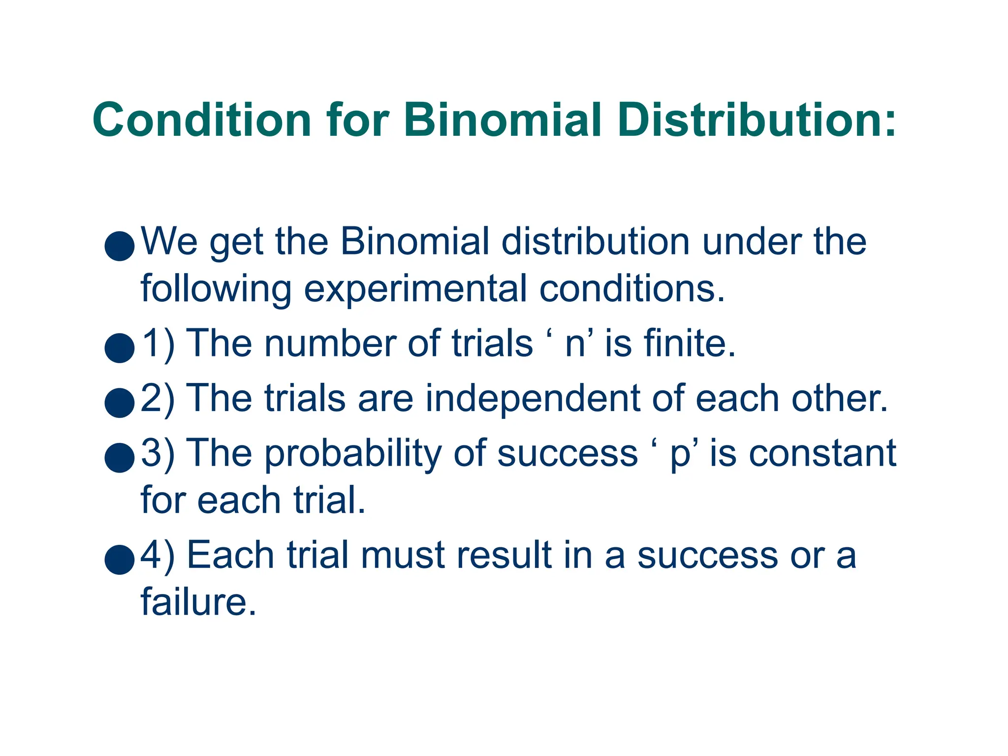
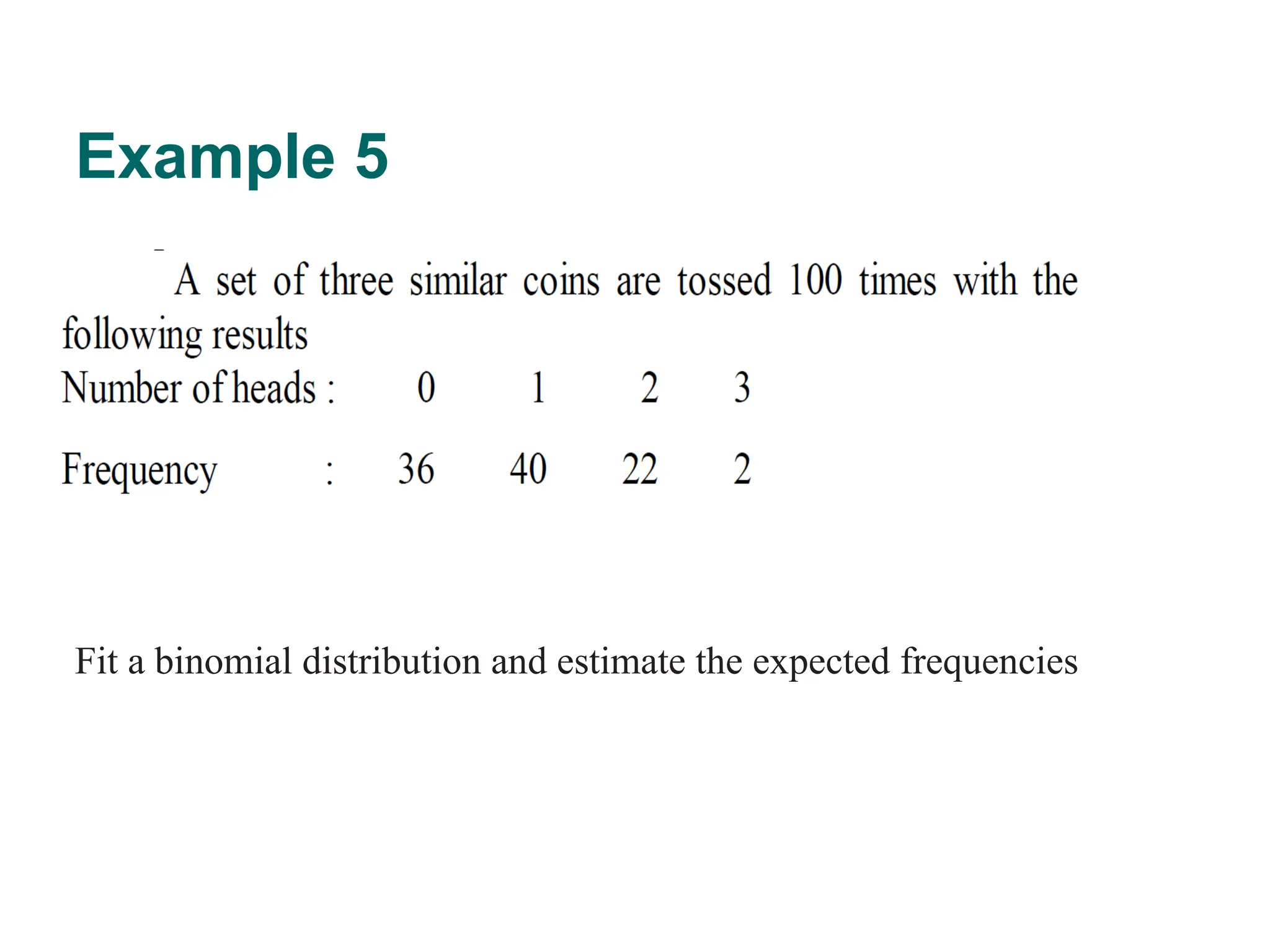
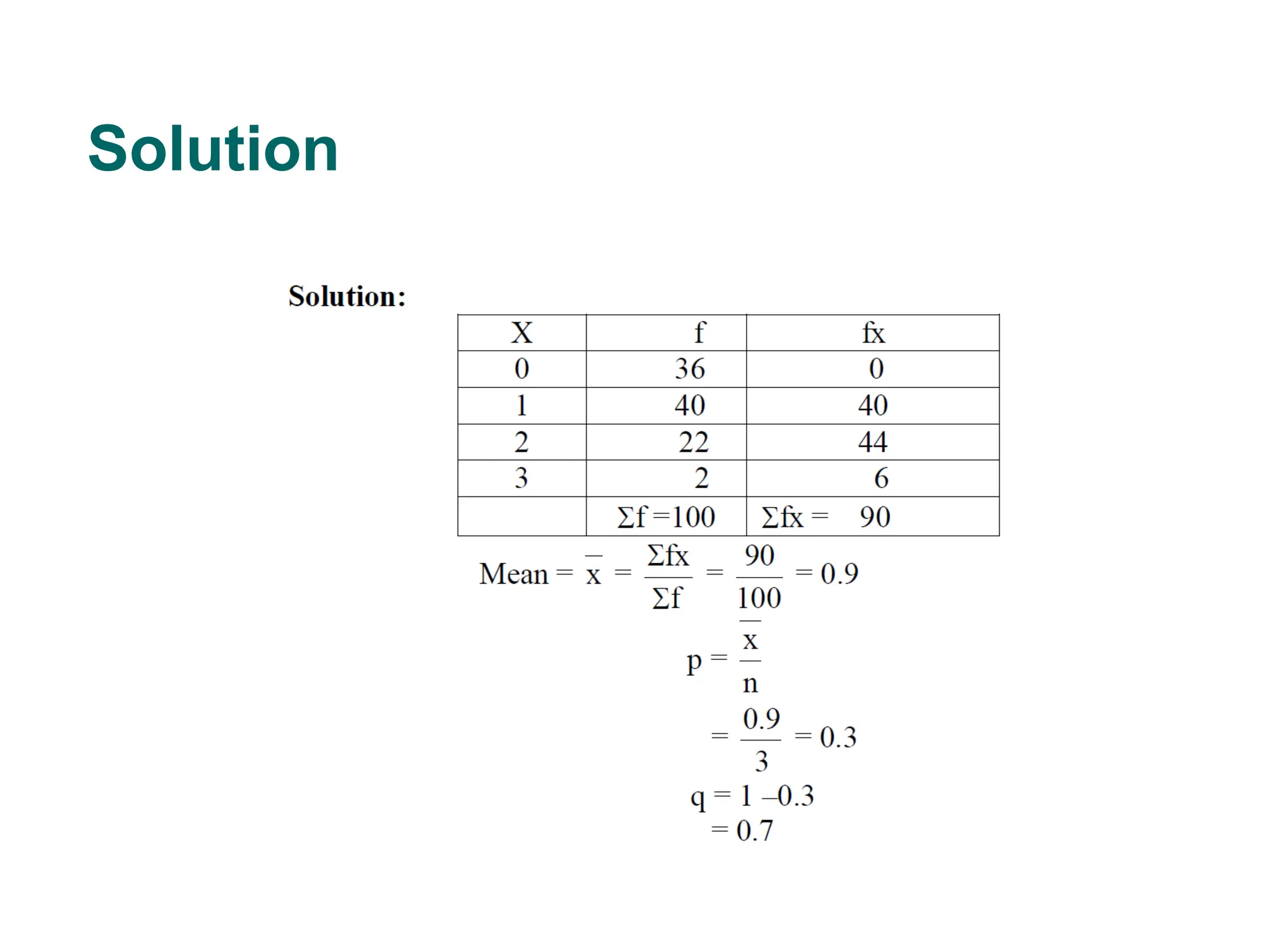
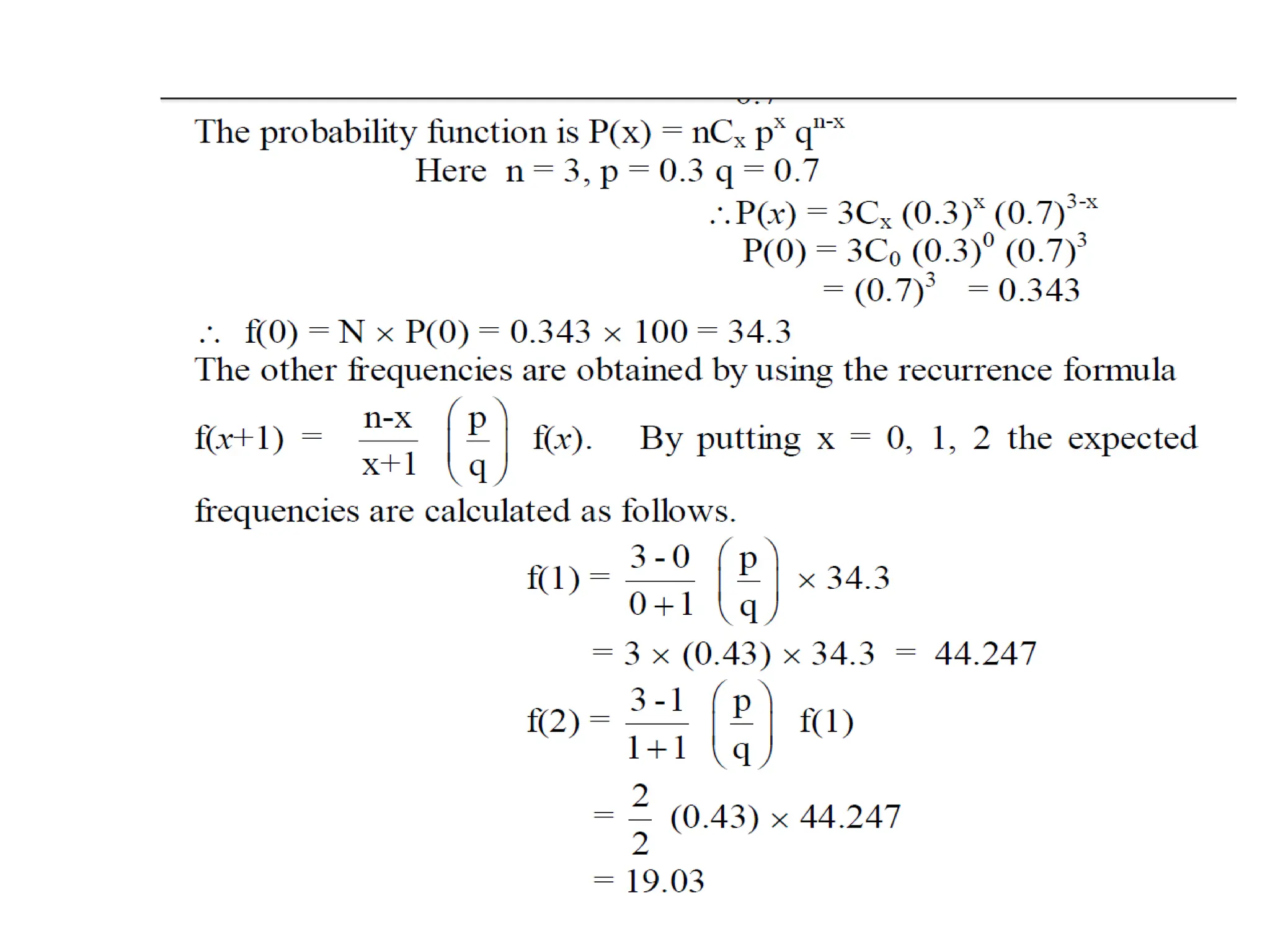
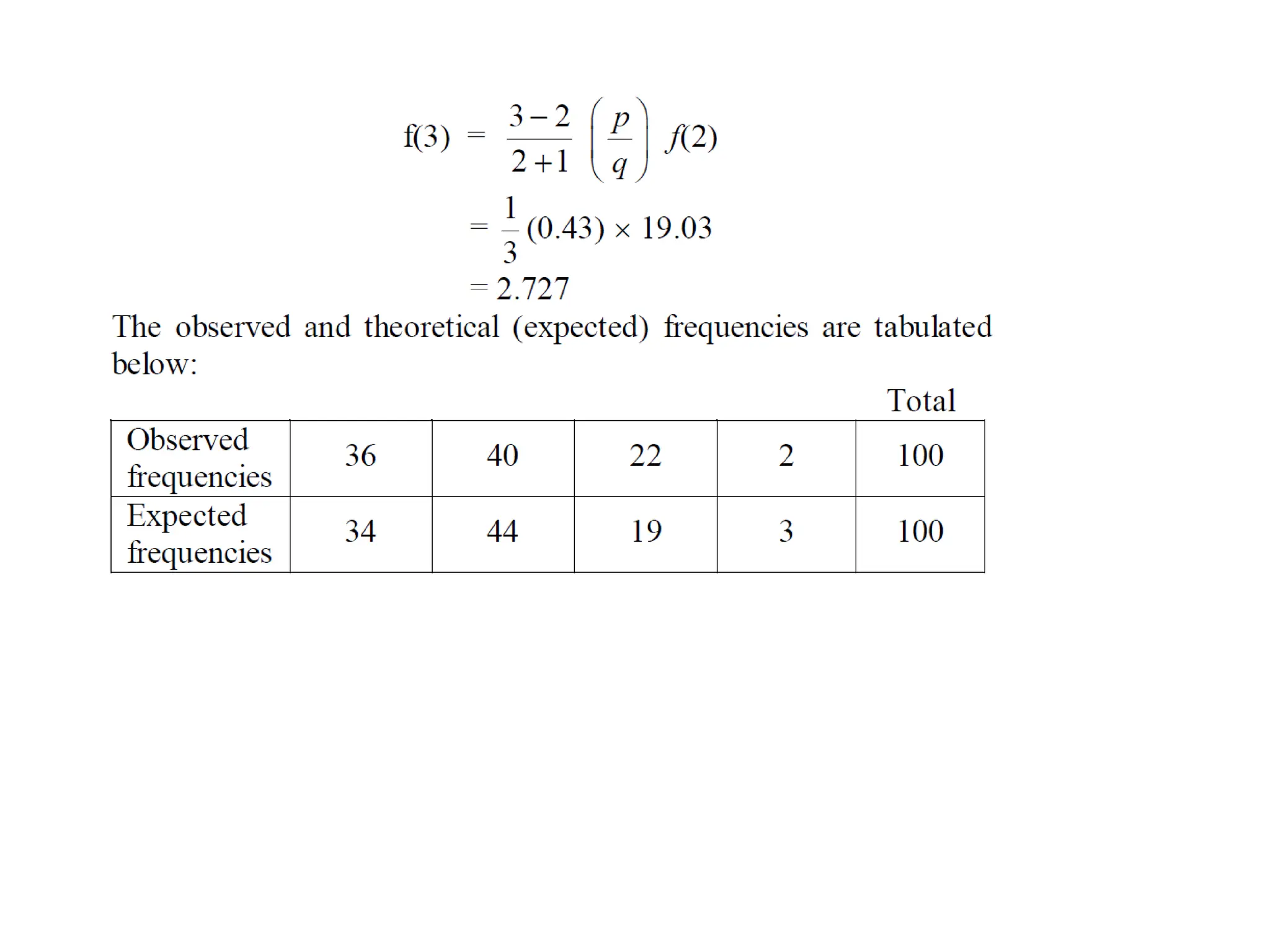
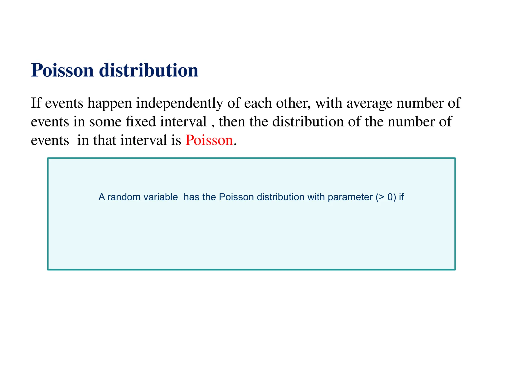
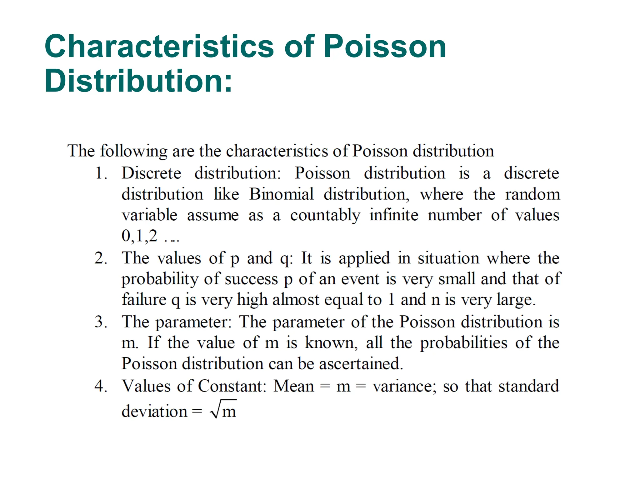
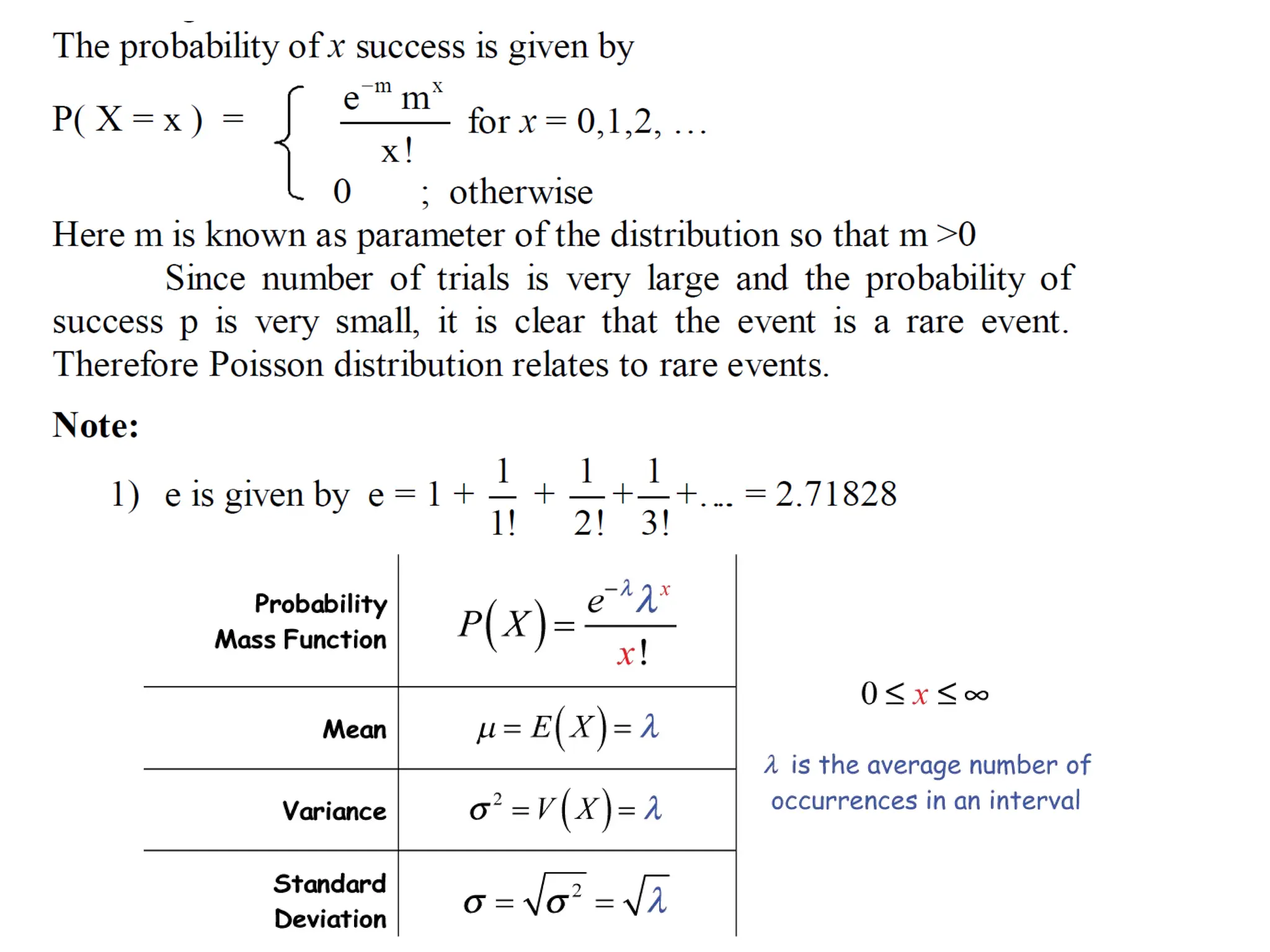
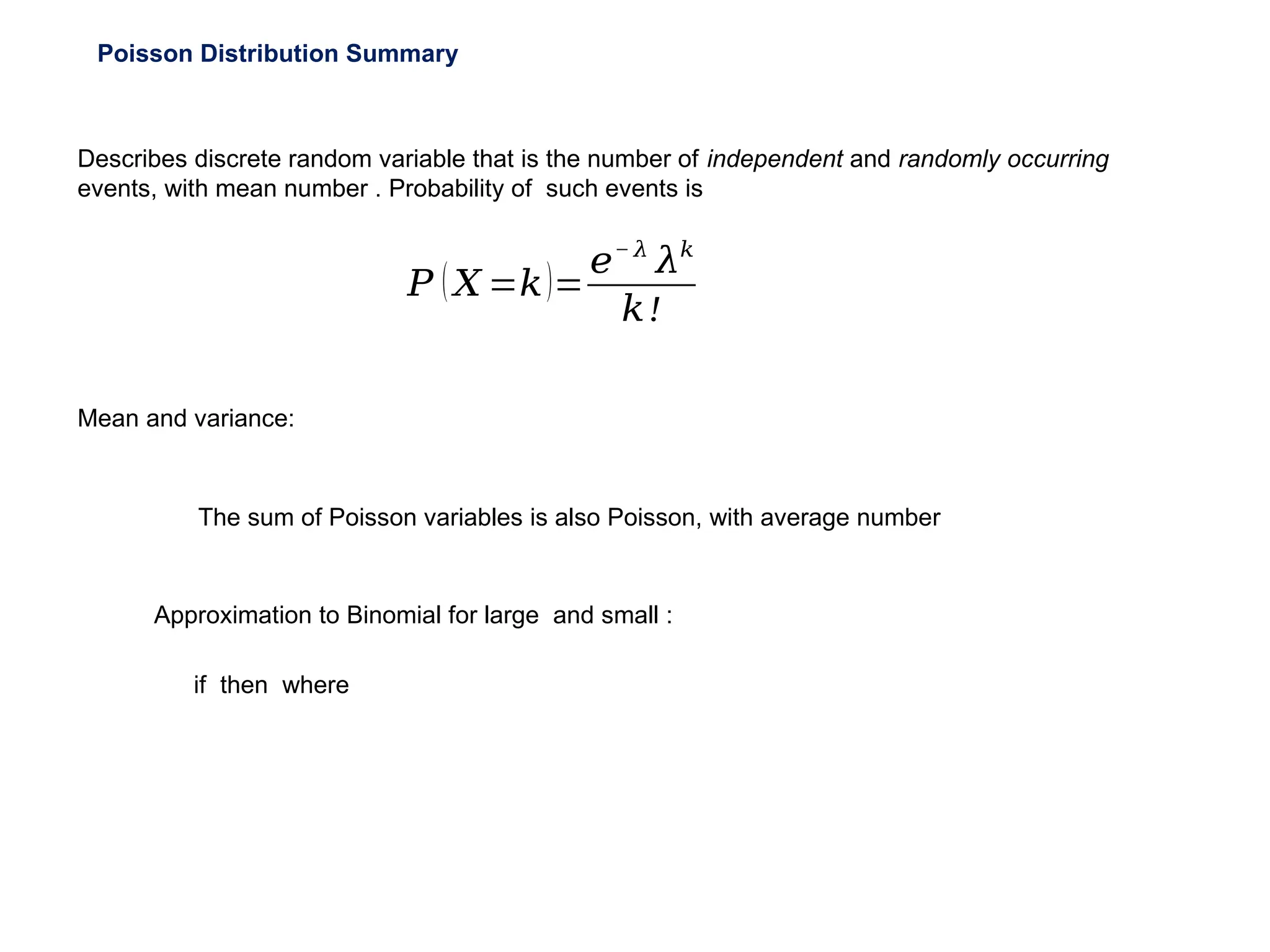
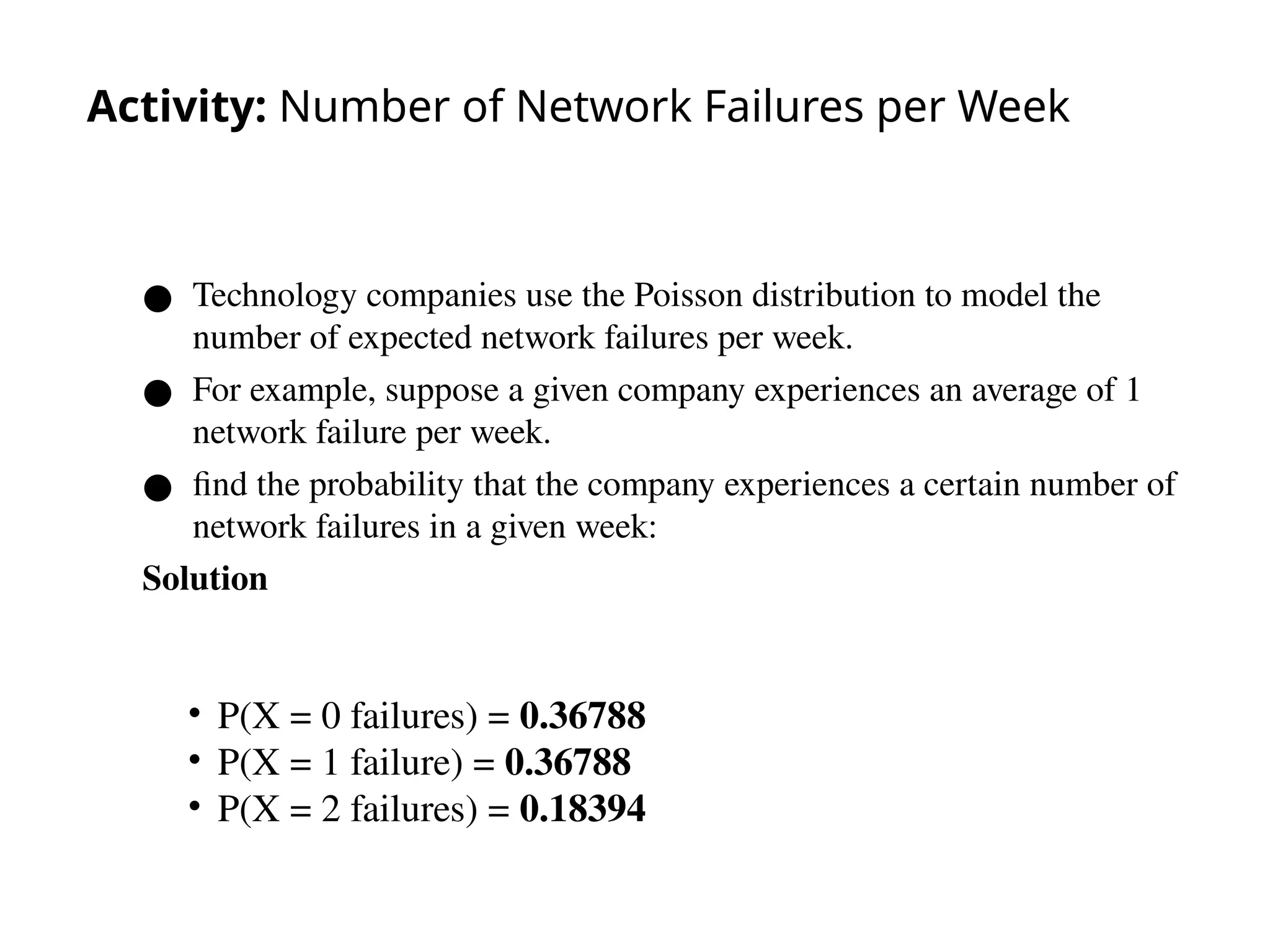
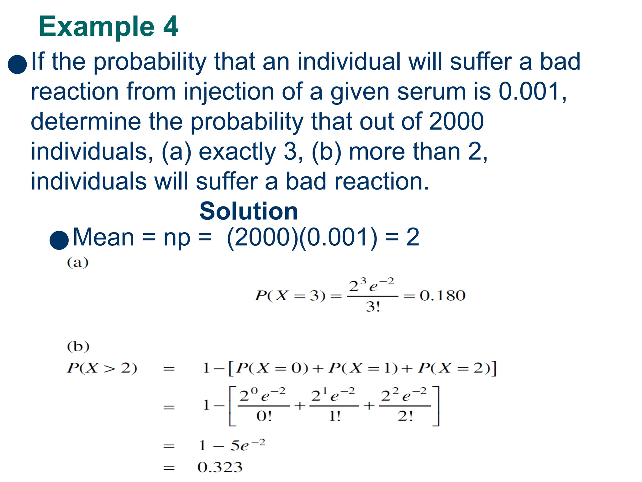
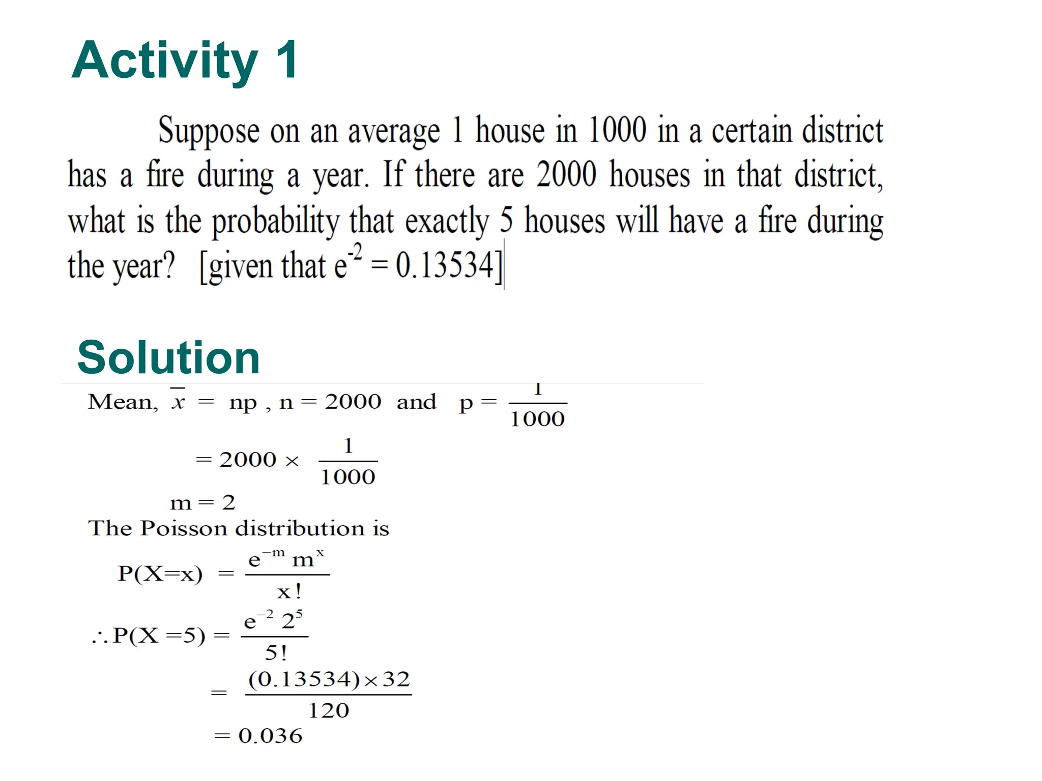
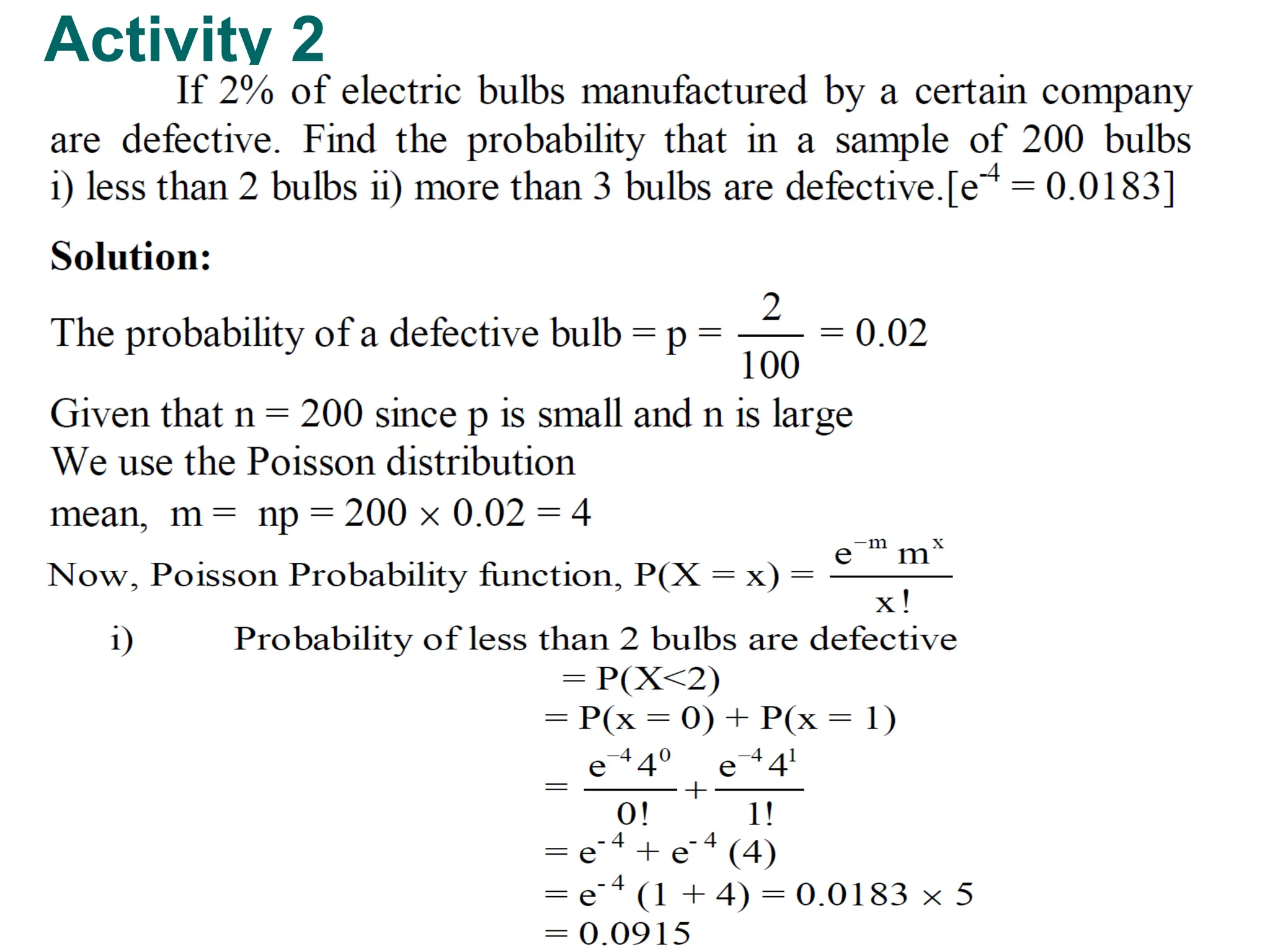
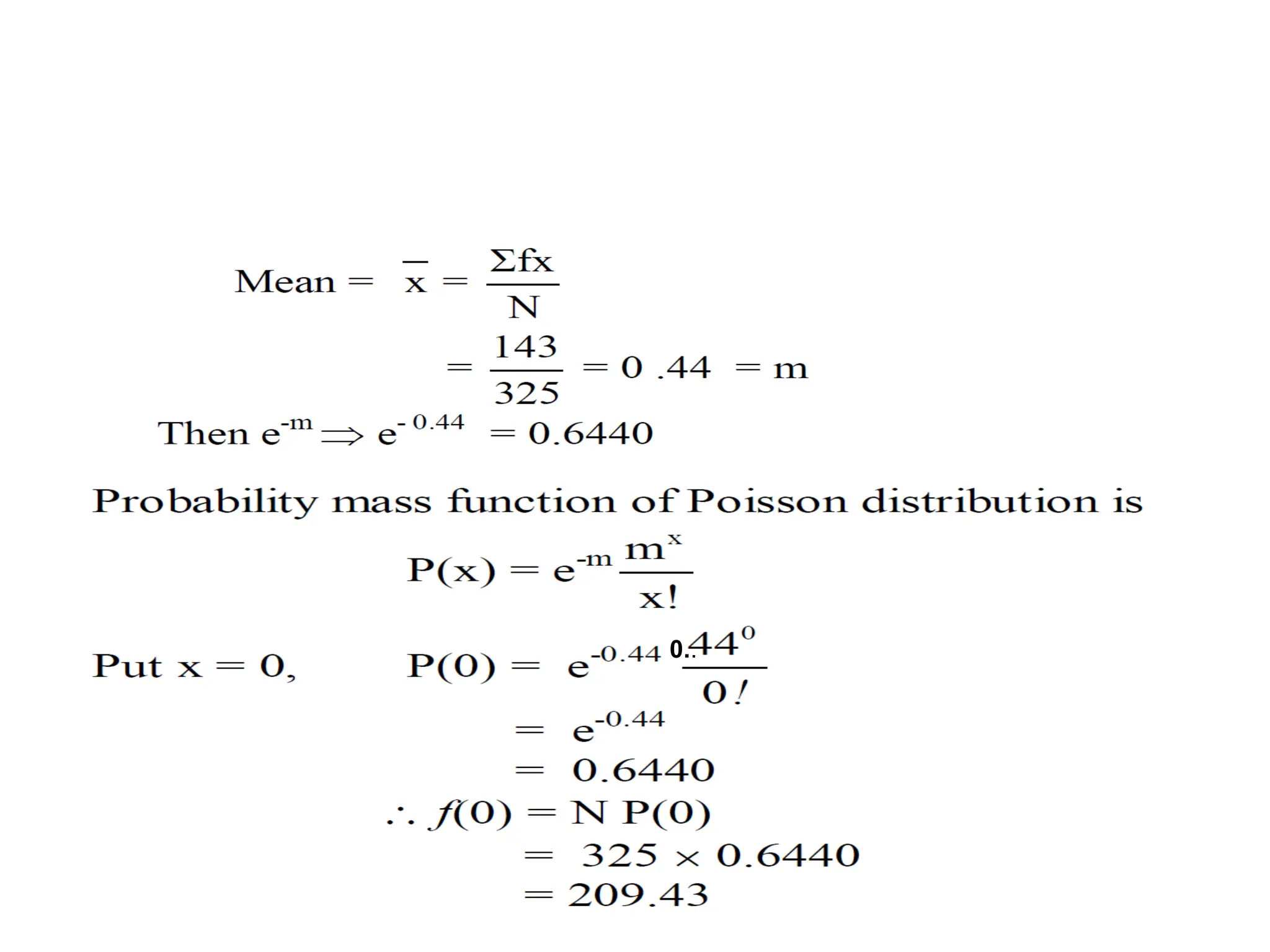
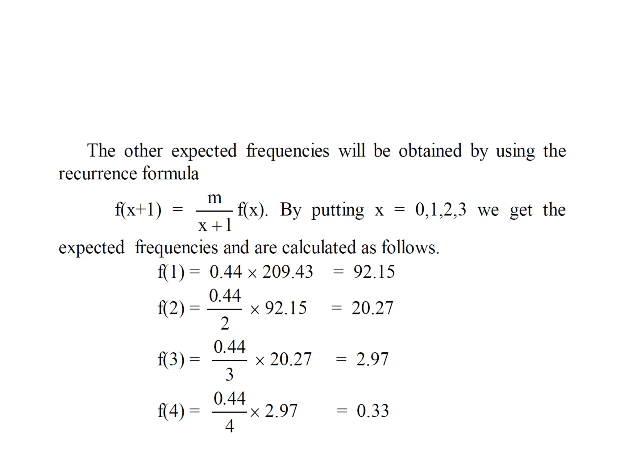
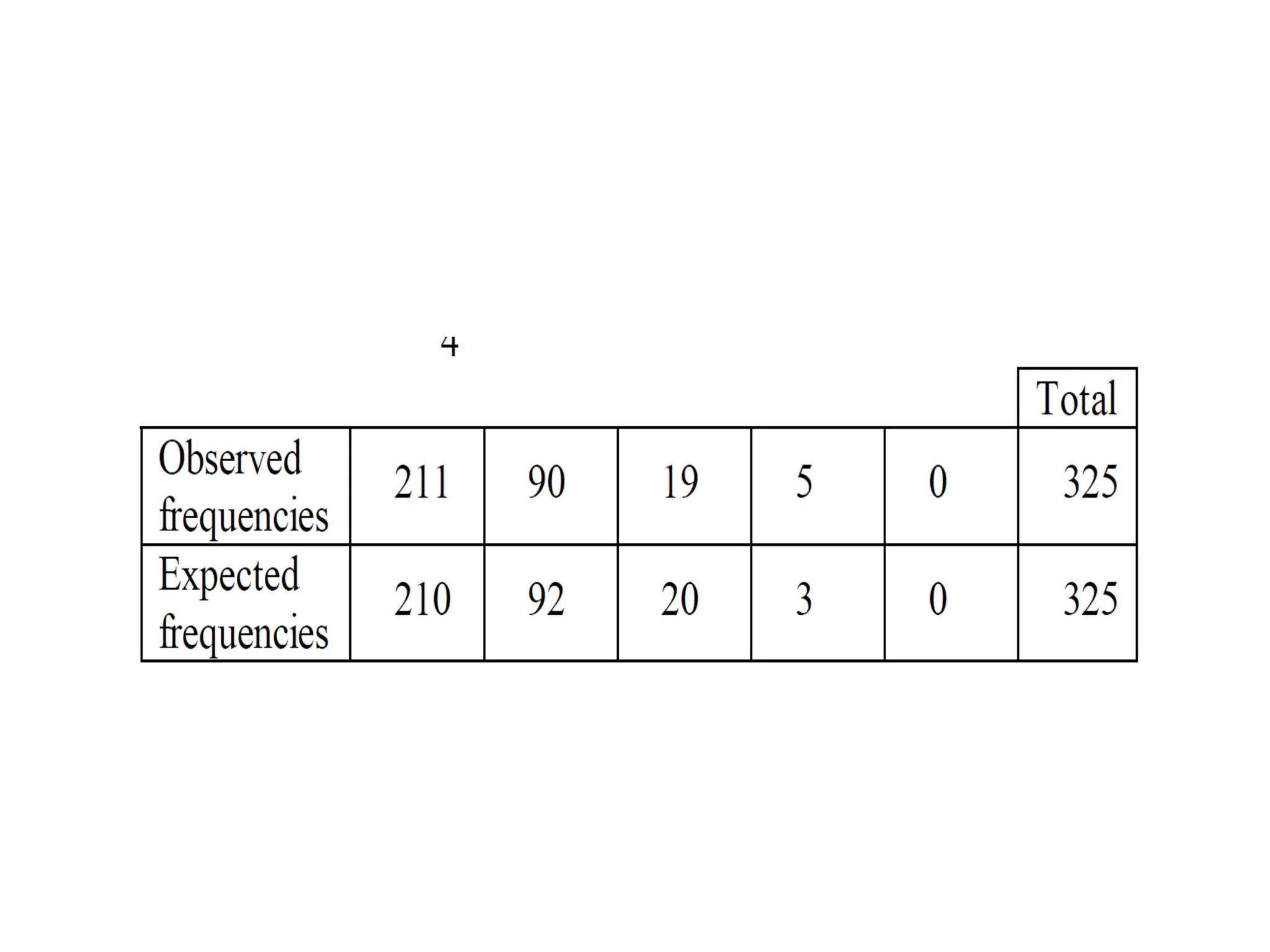
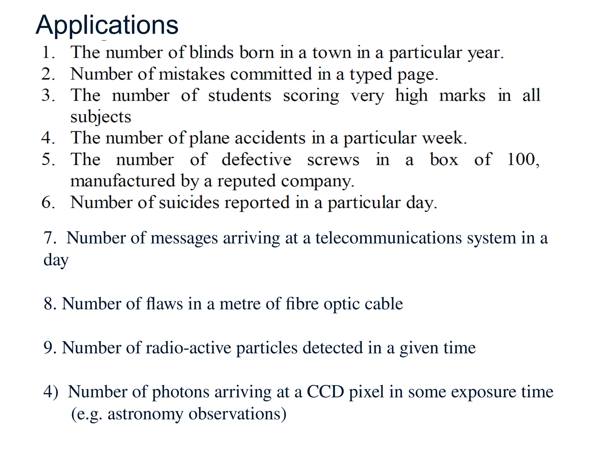
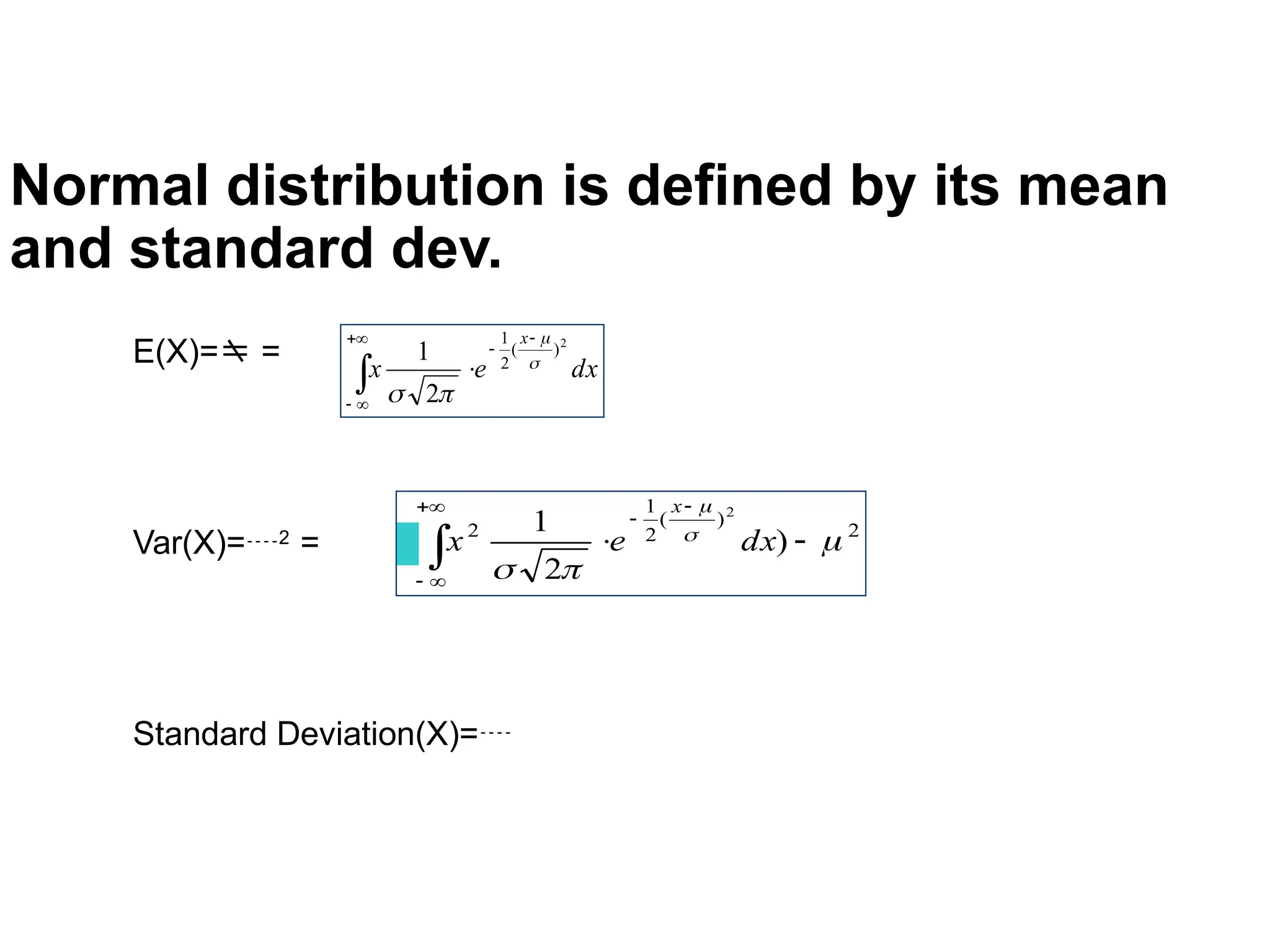
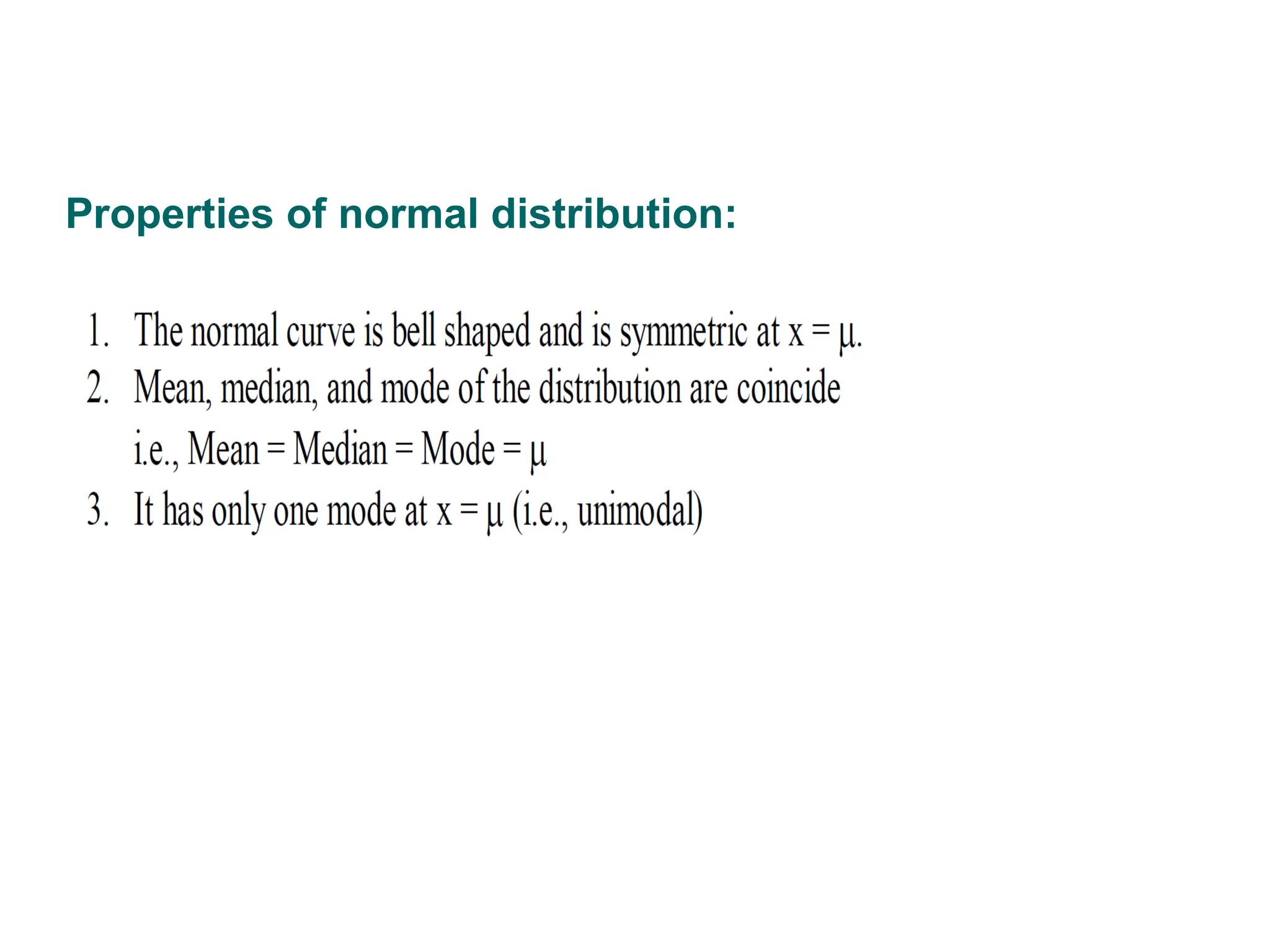
The document discusses several important theoretical distributions in probability and statistics, including the binomial, Poisson, and normal distributions. It covers definitions, properties, applications, and various examples for each distribution, illustrating their practical use in fields such as military, telecommunications, and other industries. Key concepts like Bernoulli trials, mean, variance, and the empirical rule for normal distribution are also highlighted.