Probability Distribution of its types, Z test, and sums

1. By
Abhishek Darge 70
Punit raut 98
Shriya singh 109
Priti Shrivastav 111
Sameer surve 112
Chetan Vinjuda 116

2. Probability Distribution
• A probability distribution describes how the outcome of an
experiment are expected to vary
• Since such distribution deals with expectation, they provide
useful models in making inferences and decision in the face of
uncertainty

3. Q1
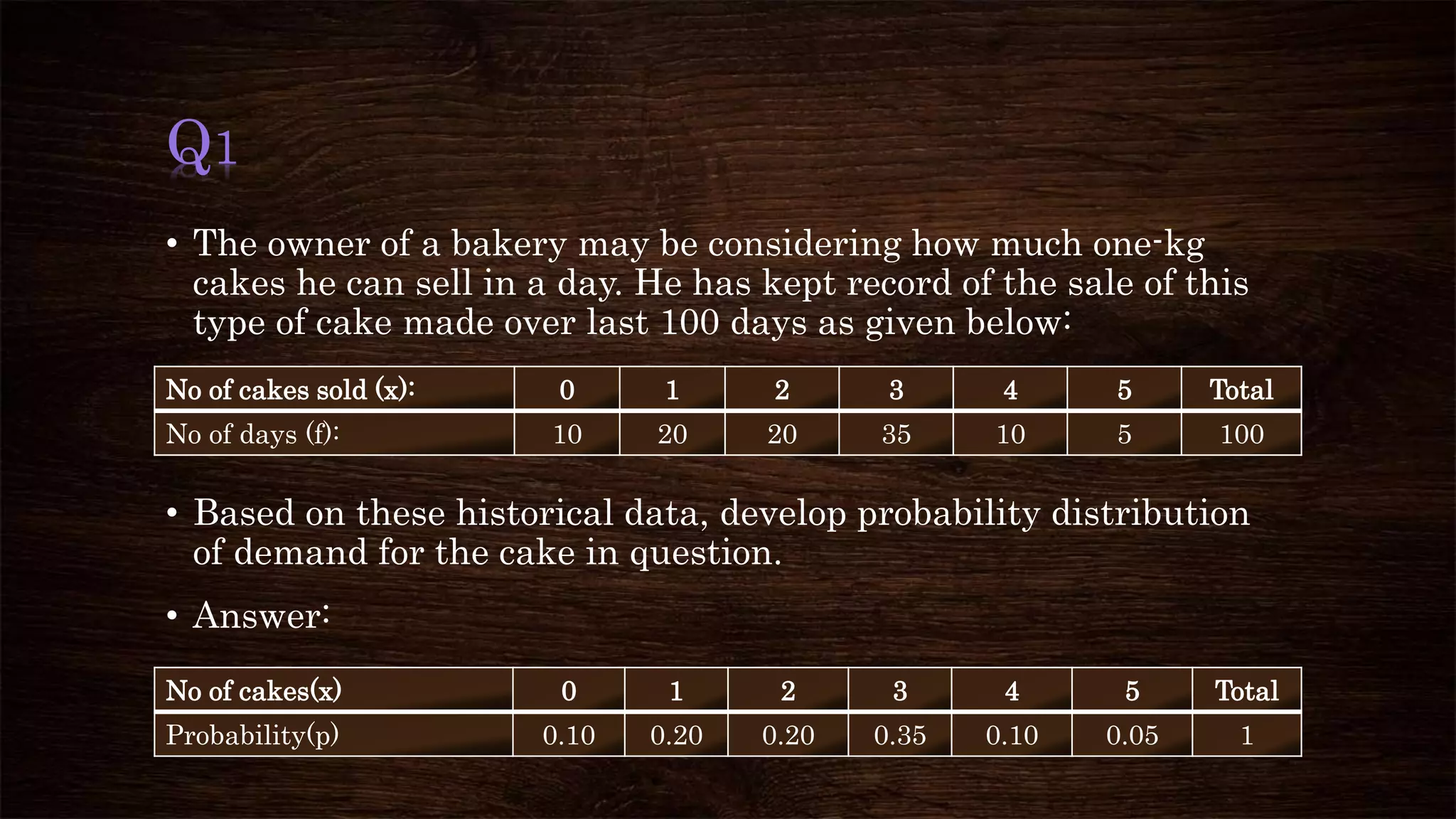
• The owner of a bakery may be considering how much one-kg
cakes he can sell in a day. He has kept record of the sale of this
type of cake made over last 100 days as given below:
• Based on these historical data, develop probability distribution
of demand for the cake in question.
• Answer:
No of cakes sold (x): 0 1 2 3 4 5 Total
No of days (f): 10 20 20 35 10 5 100
No of cakes(x) 0 1 2 3 4 5 Total
Probability(p) 0.10 0.20 0.20 0.35 0.10 0.05 1

4. Types of Probability Distribution
Discrete Probability Distribution
1. Binomial Distribution
2. Poisson Distribution
Continuous Probability Distribution
1. Uniform Probability Distribution
2. Exponential Probability
Distribution
3. Normal Probability Distribution
4. Student’s t Distribution
5. Chi-Square Distribution
6. F Distribution

5. Discrete Probability Distribution
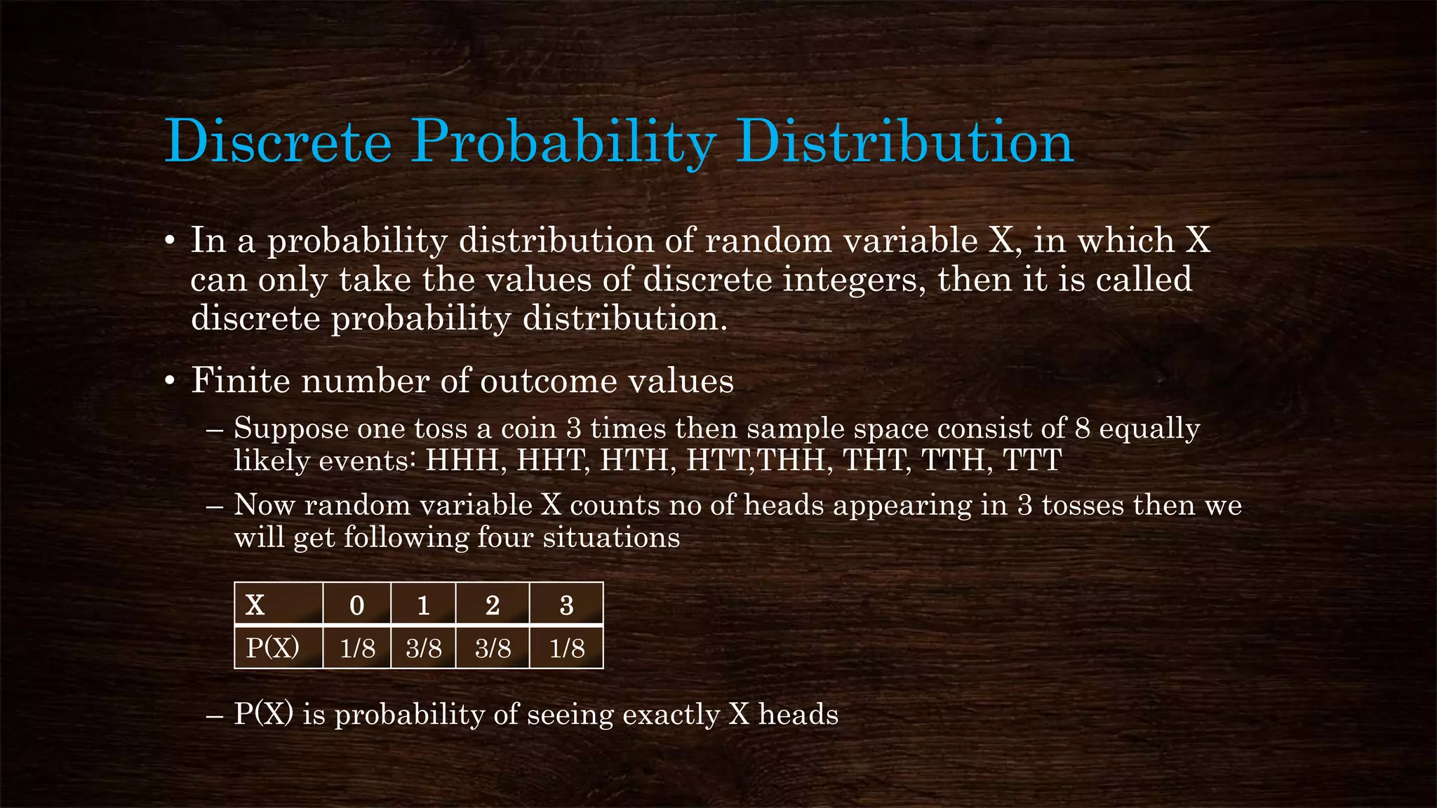
• In a probability distribution of random variable X, in which X
can only take the values of discrete integers, then it is called
discrete probability distribution.
• Finite number of outcome values
– Suppose one toss a coin 3 times then sample space consist of 8 equally
likely events: HHH, HHT, HTH, HTT,THH, THT, TTH, TTT
– Now random variable X counts no of heads appearing in 3 tosses then we
will get following four situations
– P(X) is probability of seeing exactly X heads
X 0 1 2 3
P(X) 1/8 3/8 3/8 1/8

6. Continuous Probability Distribution
• The probability distribution of a random variable is called
Continuous Probability Distribution if the given random variable
is continuous.
• Large number of outcomes
• Suppose that the Indian air force sets the qualification that all
pilots must weight between 55kg and 65kg. Then the weight of
pilot would be an example of continuous variable. Since pilot’s
weight could take any value between 55kg and 65kg

7. Binomial Distribution
• Binomial distribution takes place when there are only two
mutually exclusive possible outcomes.
• E.g.: Flipping a coin

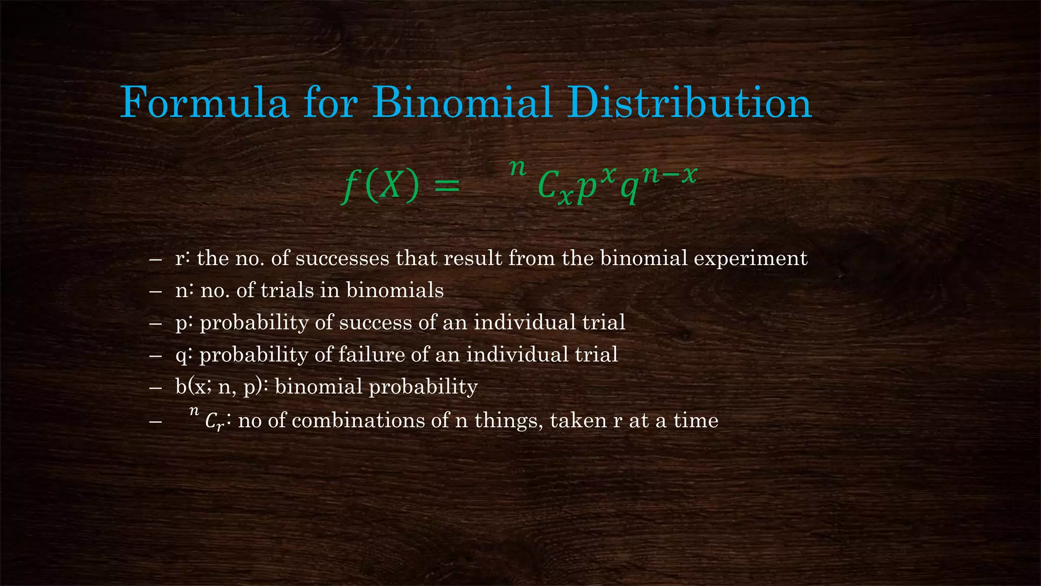
8. Formula for Binomial Distribution
𝑓 𝑋 =
𝑛
𝐶 𝑥 𝑝 𝑥
𝑞 𝑛−𝑥
– r: the no. of successes that result from the binomial experiment
– n: no. of trials in binomials
– p: probability of success of an individual trial
– q: probability of failure of an individual trial
– b(x; n, p): binomial probability
–
𝑛
𝐶𝑟: no of combinations of n things, taken r at a time

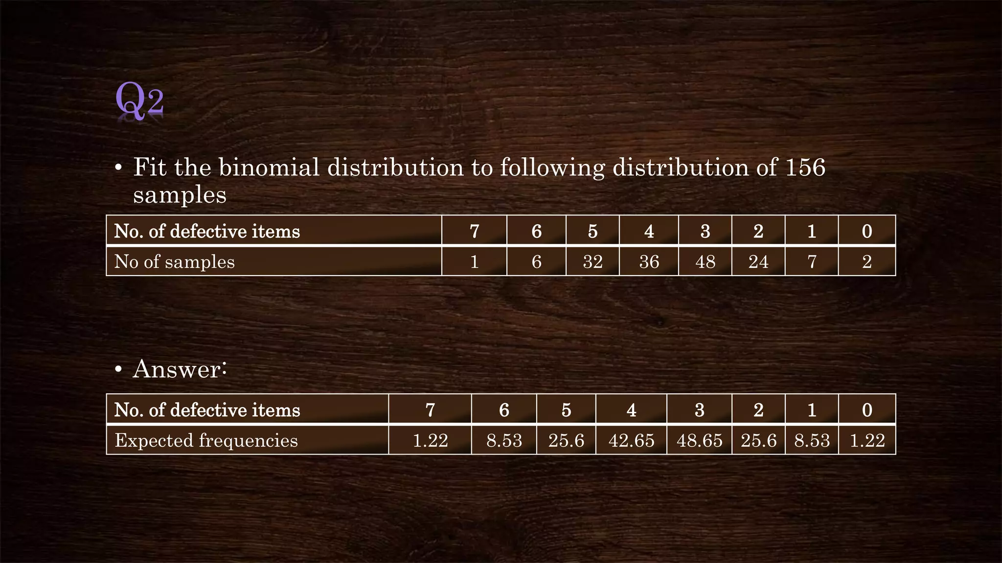
9. Q2
• Fit the binomial distribution to following distribution of 156
samples
• Answer:
No. of defective items 7 6 5 4 3 2 1 0
No of samples 1 6 32 36 48 24 7 2
No. of defective items 7 6 5 4 3 2 1 0
Expected frequencies 1.22 8.53 25.6 42.65 48.65 25.6 8.53 1.22

10. Poisson Distribution
• Poisson distribution is discrete random variable distribution that
expresses probability of given number of event in a fix interval of
time, if these event occur with a known average rate and
independent of the time since the last event.
• It can be used as an alternative to binominal distribution in case
of very large sample
• E.g.
– No of accidents per year in a district of Maharashtra
– No of typing error per page
– No of vehicles passing a certain point per minute

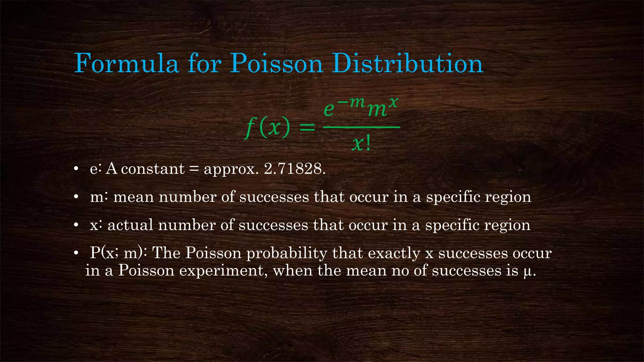
11. Formula for Poisson Distribution
𝑓 𝑥 =
𝑒−𝑚
𝑚 𝑥
𝑥!
• e: A constant = approx. 2.71828.
• m: mean number of successes that occur in a specific region
• x: actual number of successes that occur in a specific region
• P(x; m): The Poisson probability that exactly x successes occur
in a Poisson experiment, when the mean no of successes is µ.

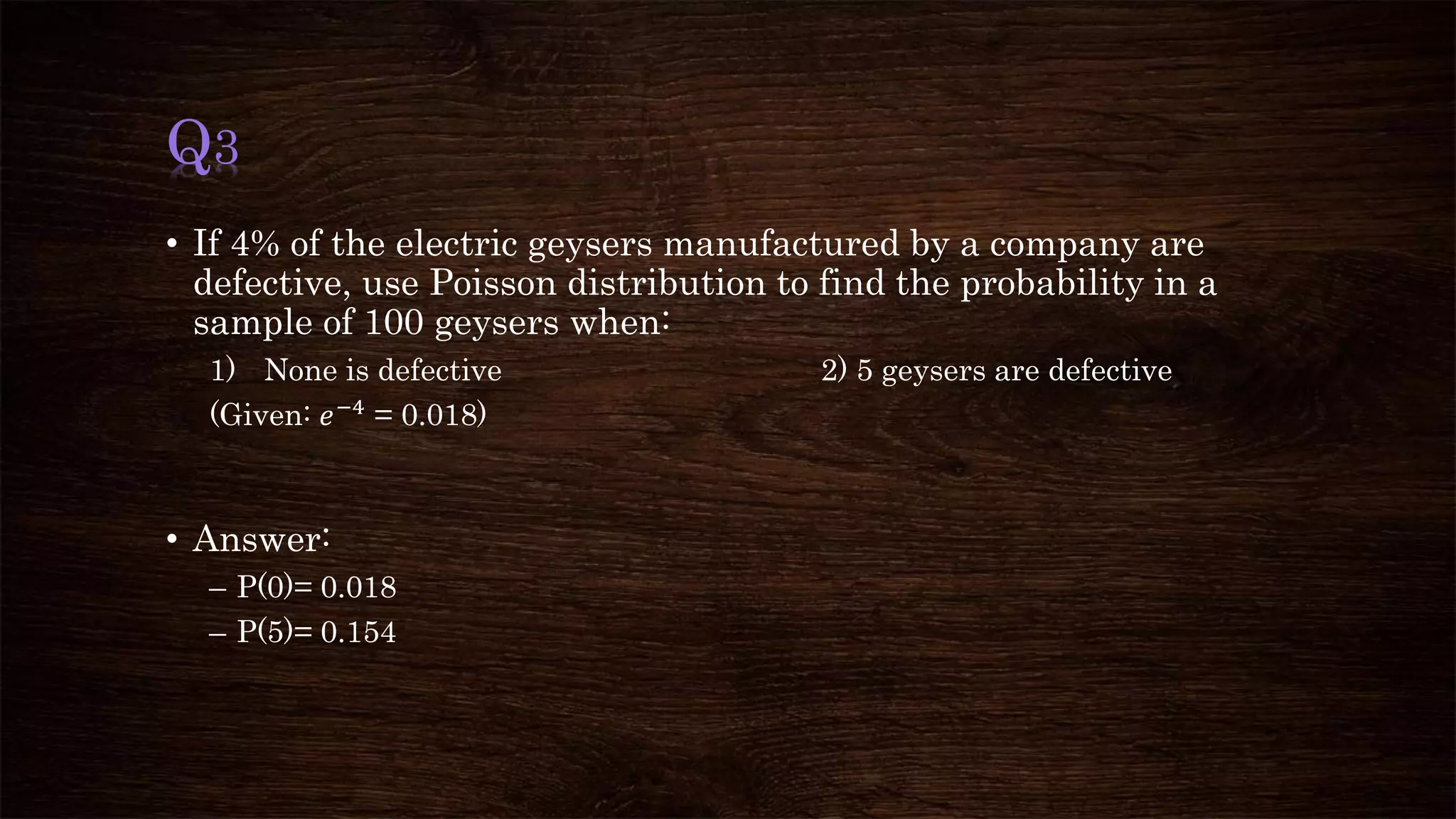
12. Q3
• If 4% of the electric geysers manufactured by a company are
defective, use Poisson distribution to find the probability in a
sample of 100 geysers when:
1) None is defective 2) 5 geysers are defective
(Given: 𝑒−4 = 0.018)
• Answer:
– P(0)= 0.018
– P(5)= 0.154

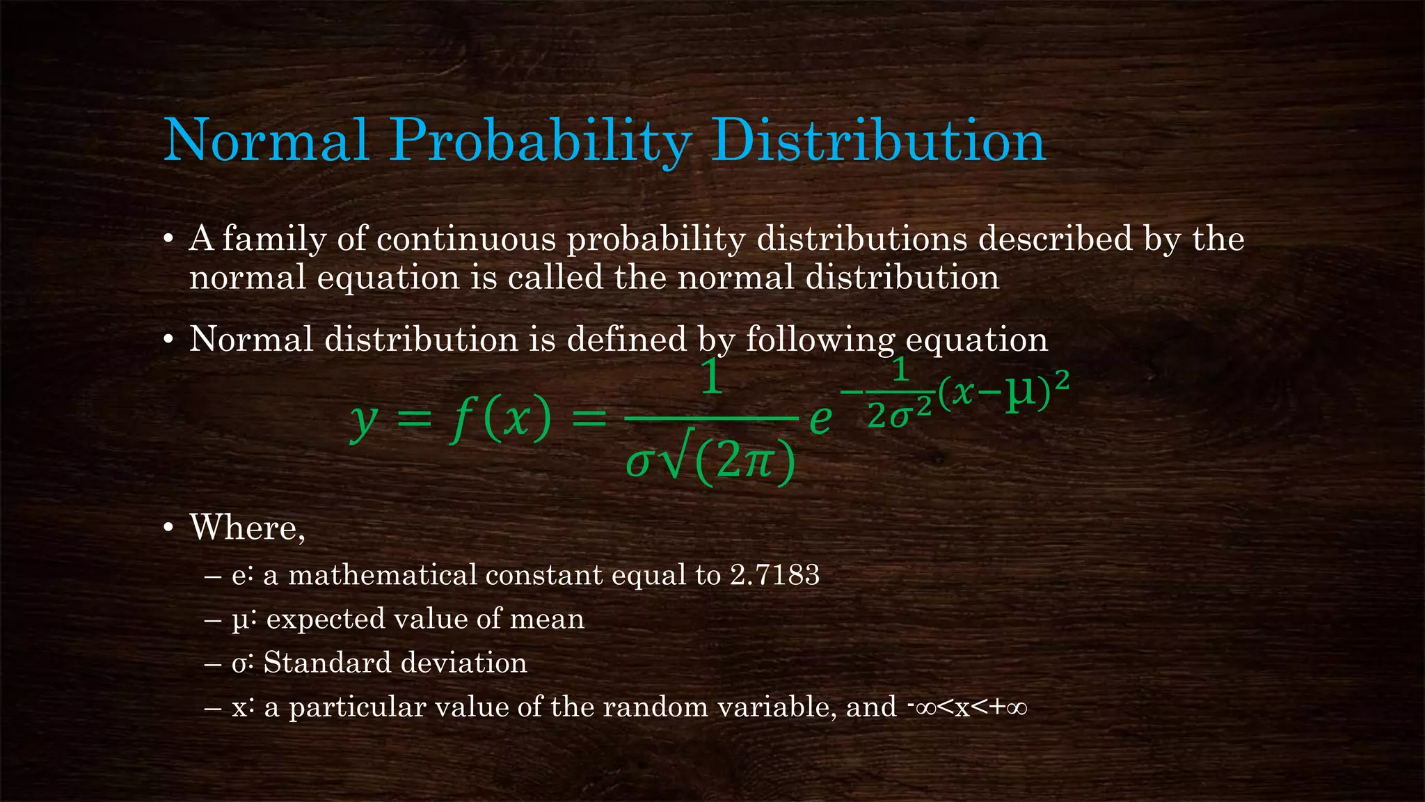
13. Normal Probability Distribution
• A family of continuous probability distributions described by the
normal equation is called the normal distribution
• Normal distribution is defined by following equation
𝑦 = 𝑓 𝑥 =
1
𝜎√(2𝜋)
𝑒
−
1
2𝜎2(𝑥−μ)2
• Where,
– e: a mathematical constant equal to 2.7183
– μ: expected value of mean
– σ: Standard deviation
– x: a particular value of the random variable, and -∞<x<+∞

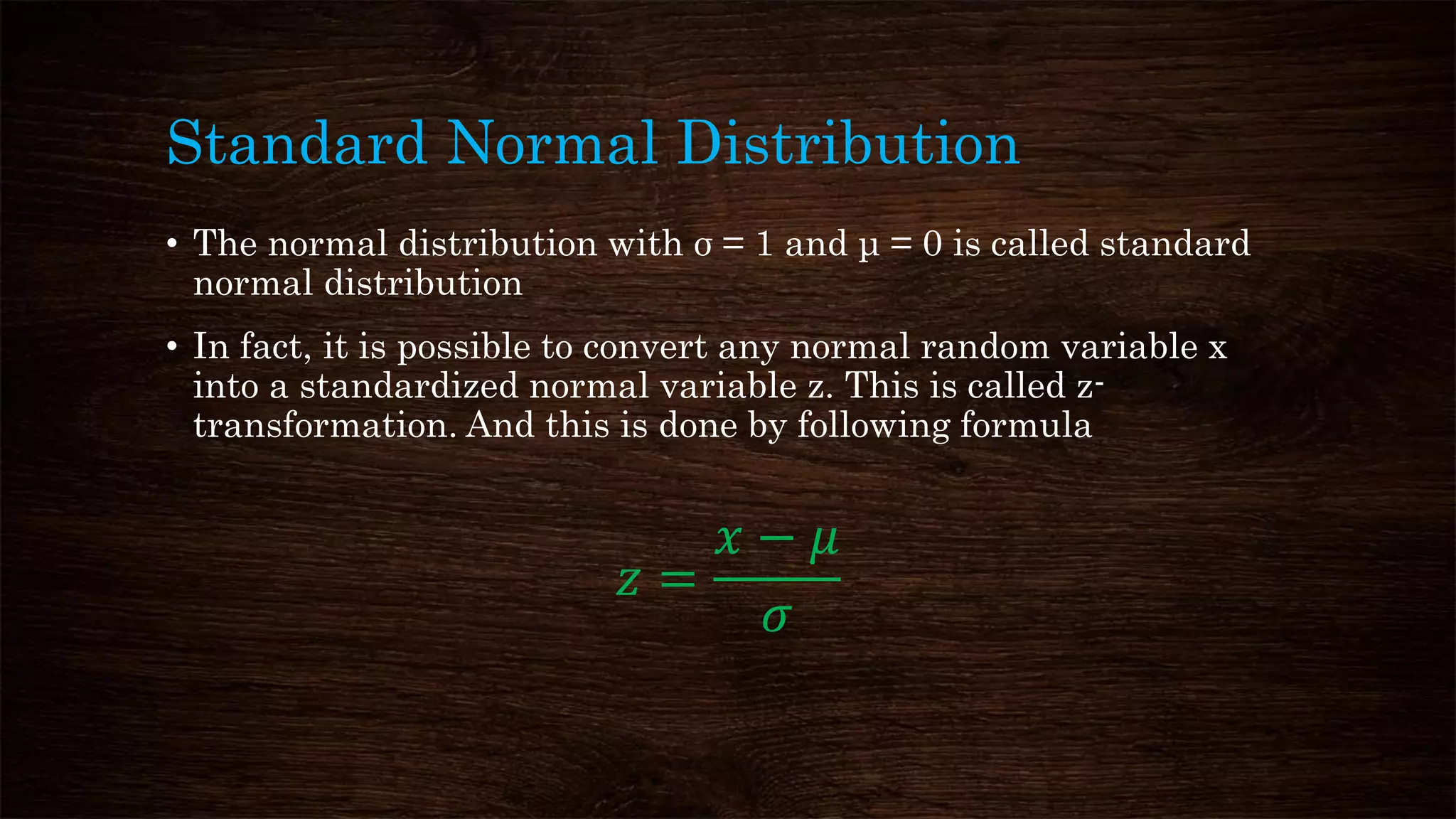
14. Standard Normal Distribution
• The normal distribution with σ = 1 and μ = 0 is called standard
normal distribution
• In fact, it is possible to convert any normal random variable x
into a standardized normal variable z. This is called z-
transformation. And this is done by following formula
𝑧 =
𝑥 − 𝜇
𝜎

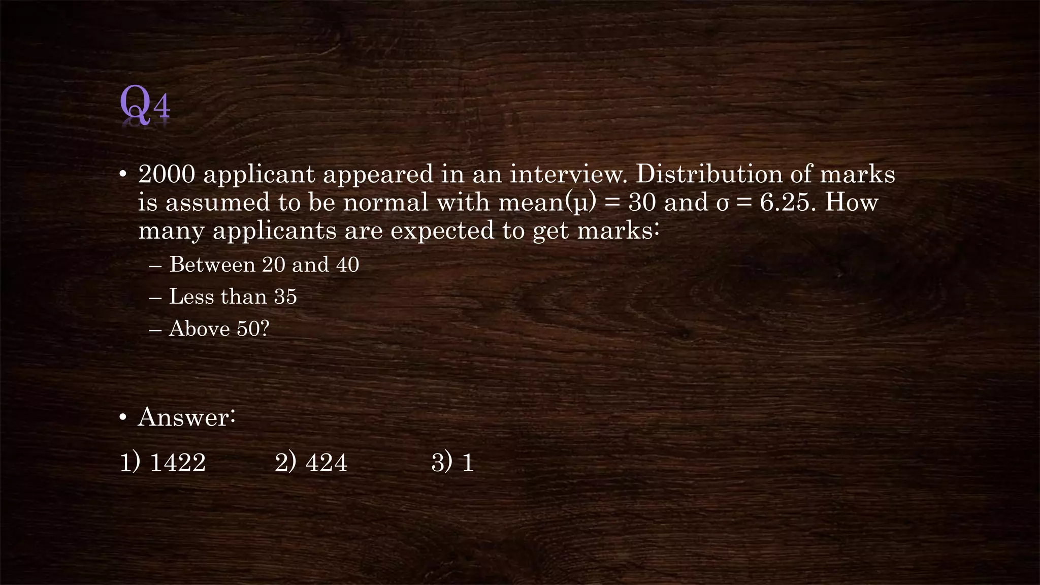
15. Q4
• 2000 applicant appeared in an interview. Distribution of marks
is assumed to be normal with mean(μ) = 30 and σ = 6.25. How
many applicants are expected to get marks:
– Between 20 and 40
– Less than 35
– Above 50?
• Answer:
1) 1422 2) 424 3) 1

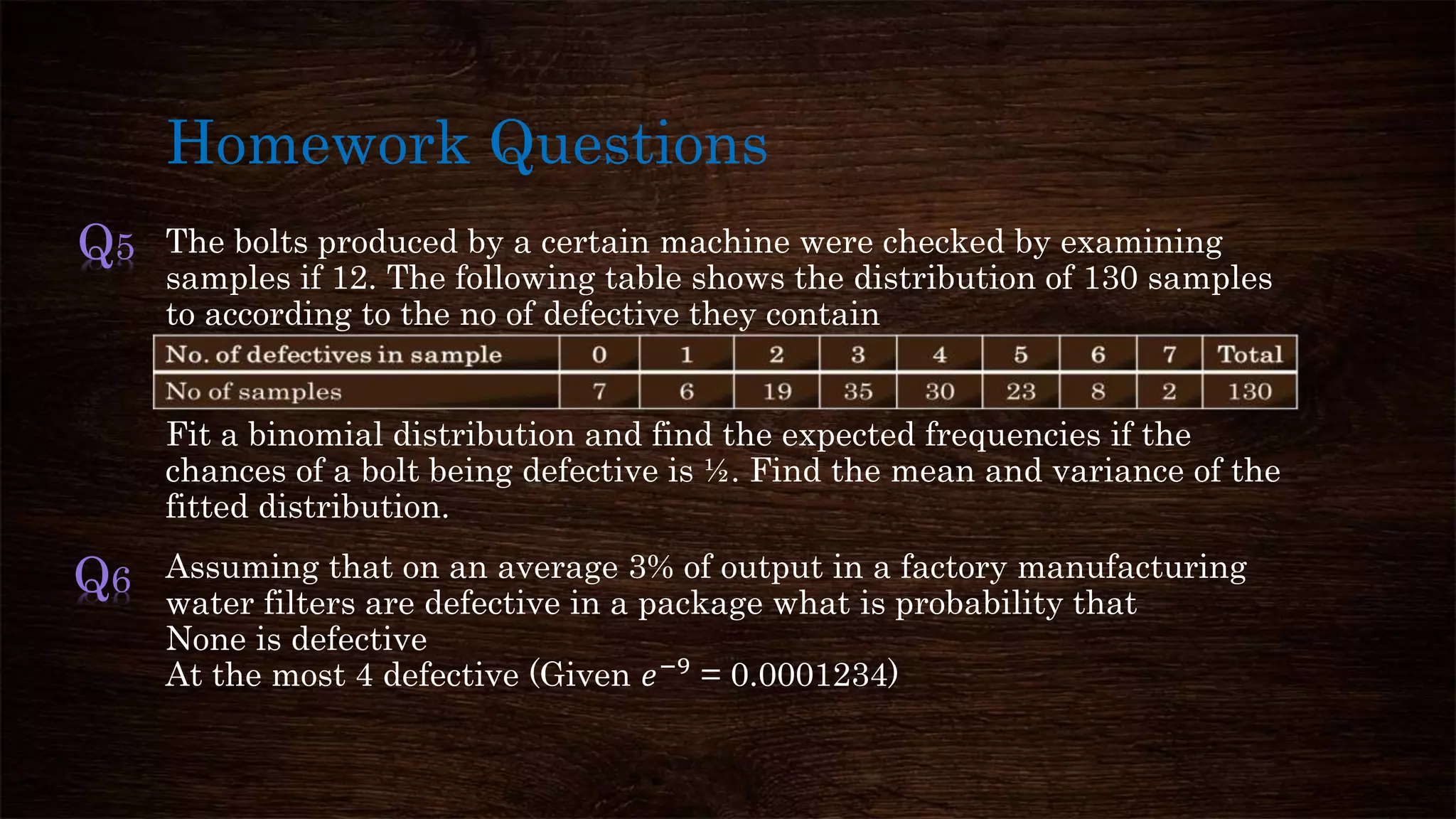
16. Homework Questions
The bolts produced by a certain machine were checked by examining
samples if 12. The following table shows the distribution of 130 samples
to according to the no of defective they contain
Fit a binomial distribution and find the expected frequencies if the
chances of a bolt being defective is ½. Find the mean and variance of the
fitted distribution.
Assuming that on an average 3% of output in a factory manufacturing
water filters are defective in a package what is probability that
None is defective
At the most 4 defective (Given 𝑒−9 = 0.0001234)
Q5
Q6