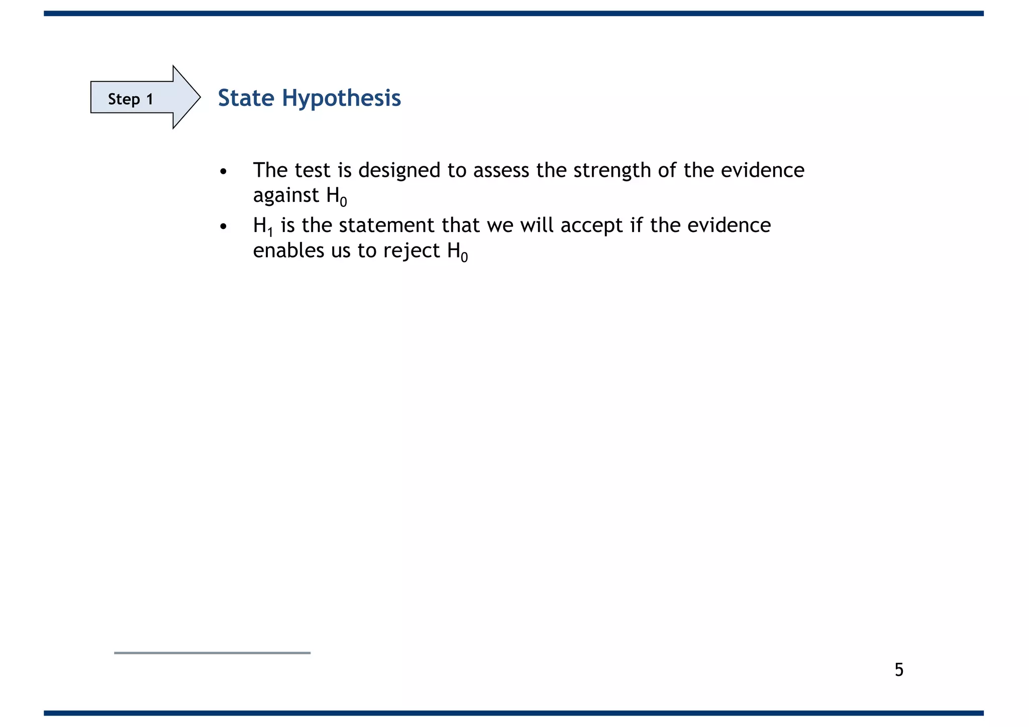
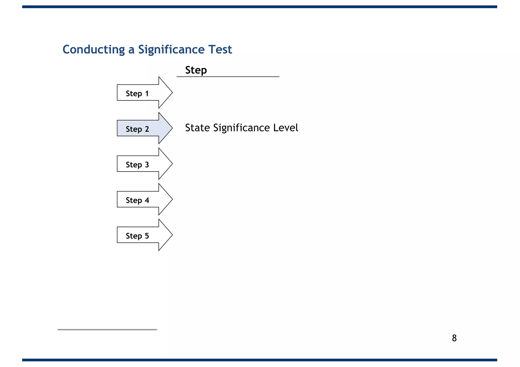
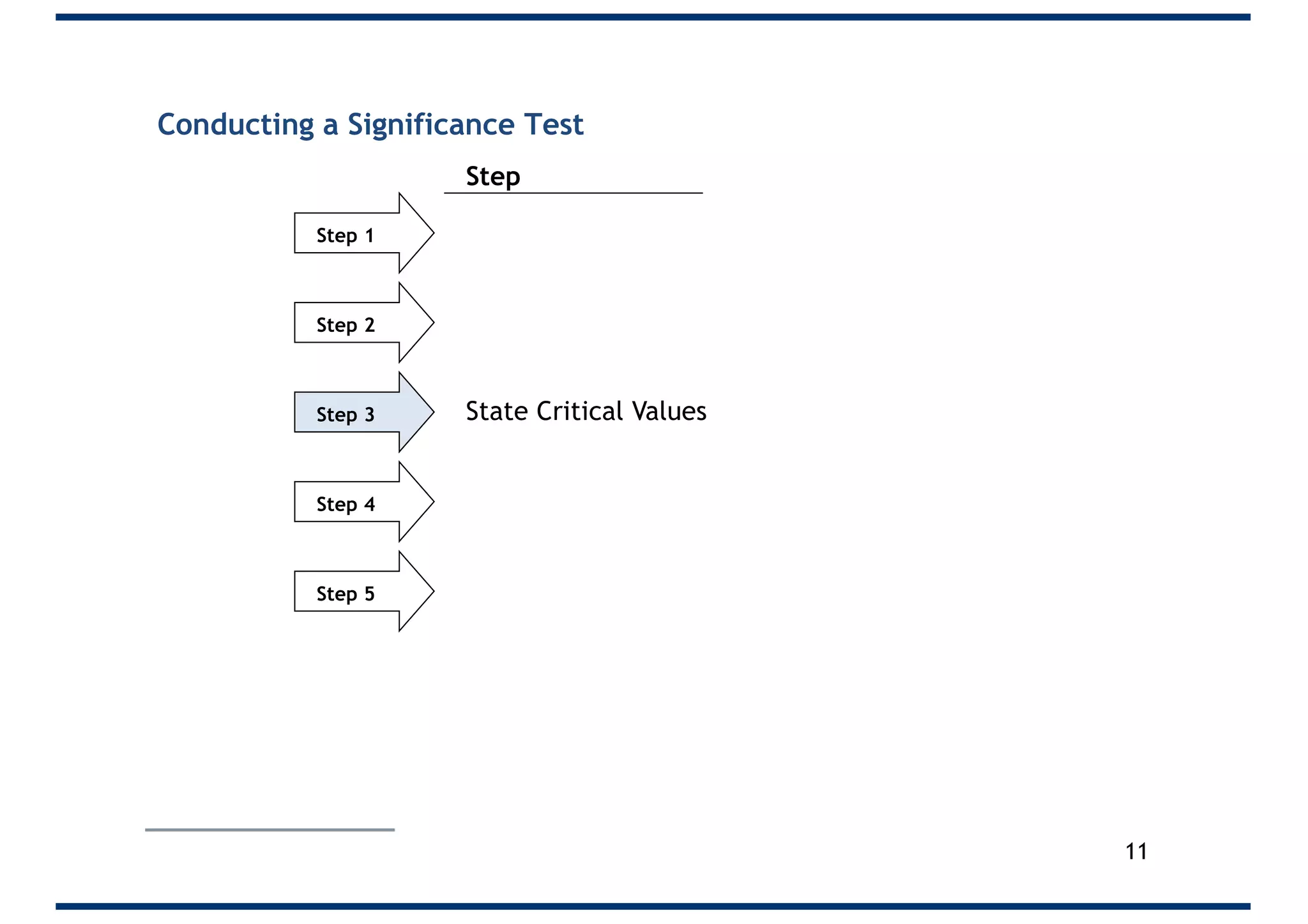
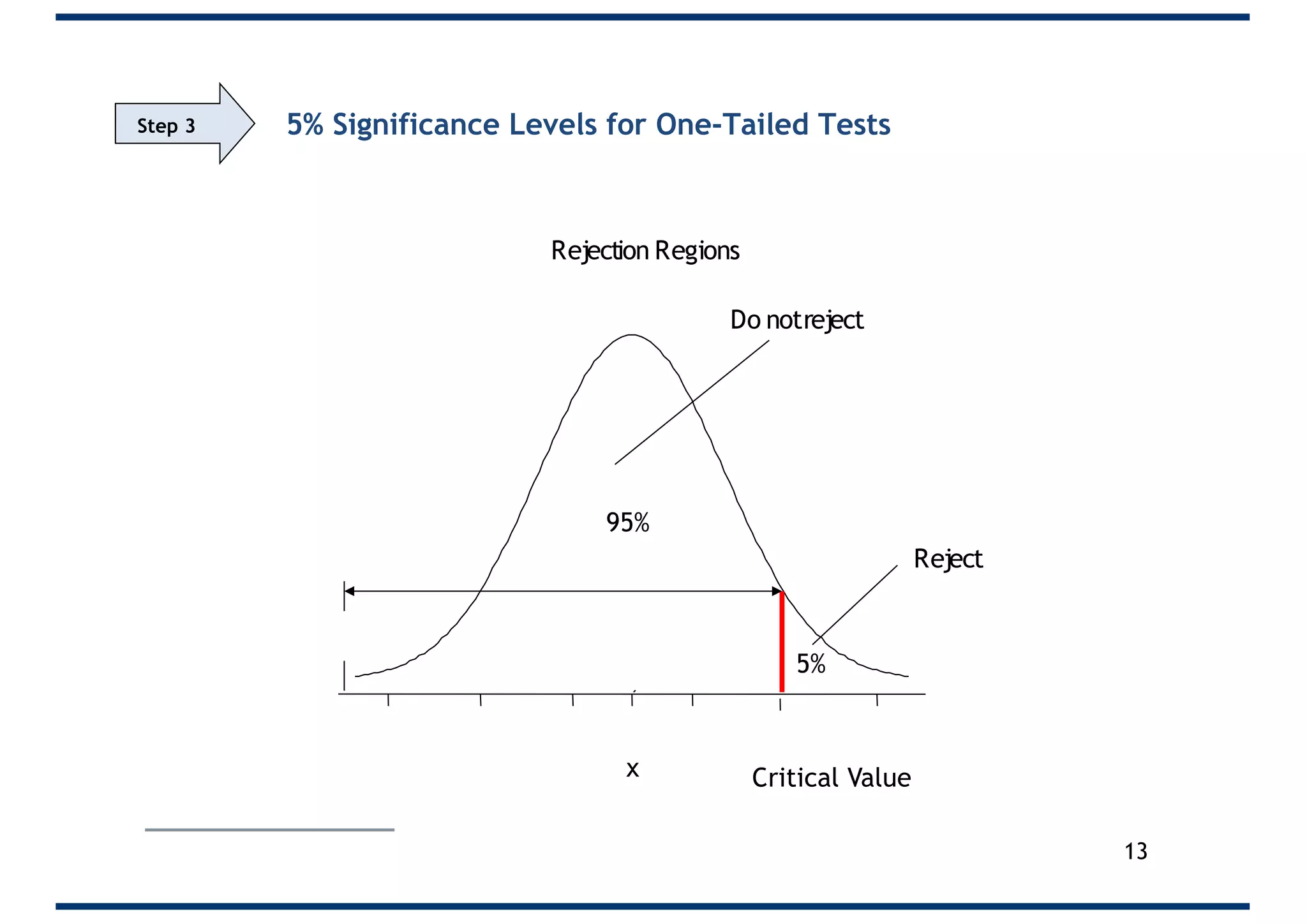
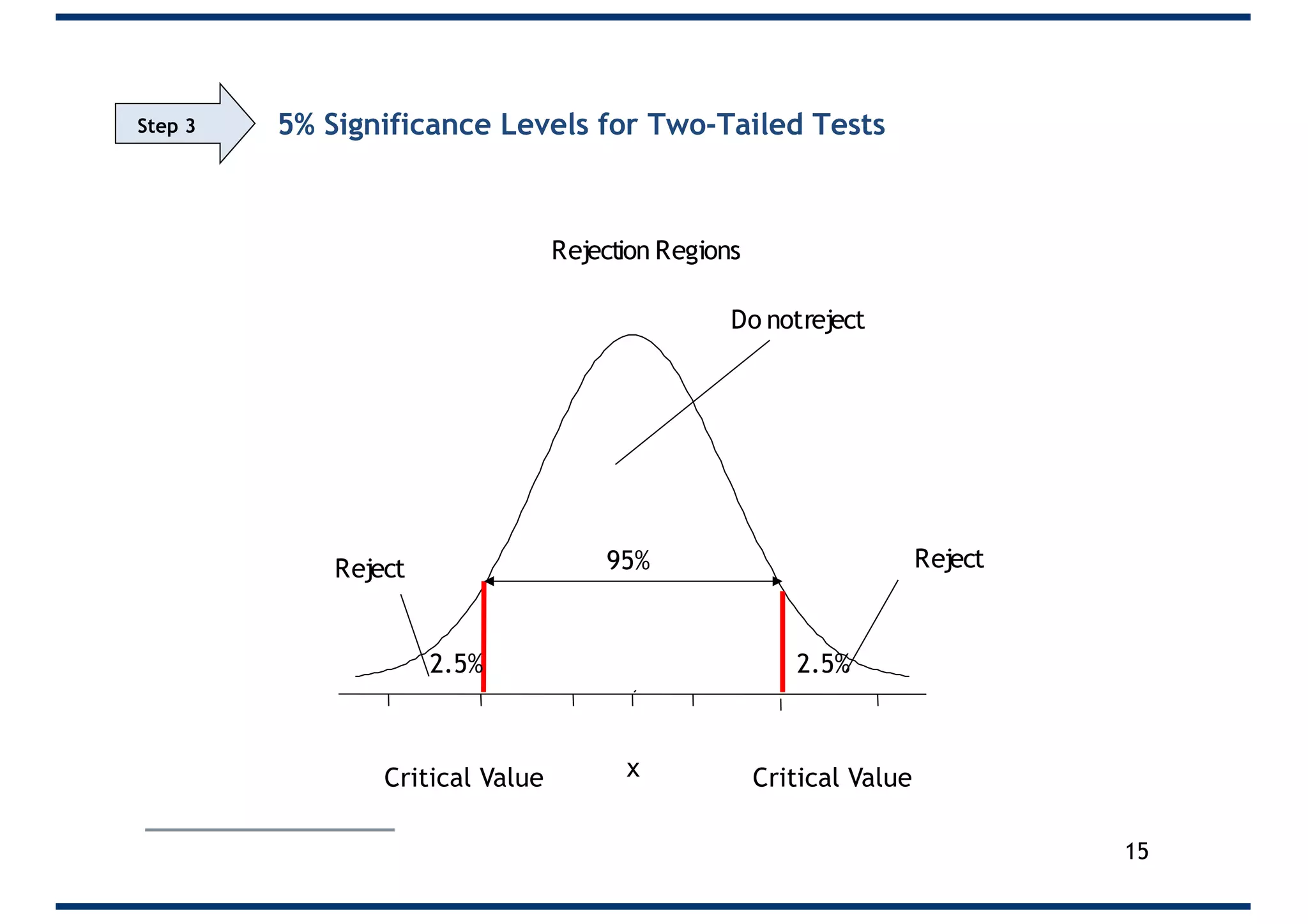
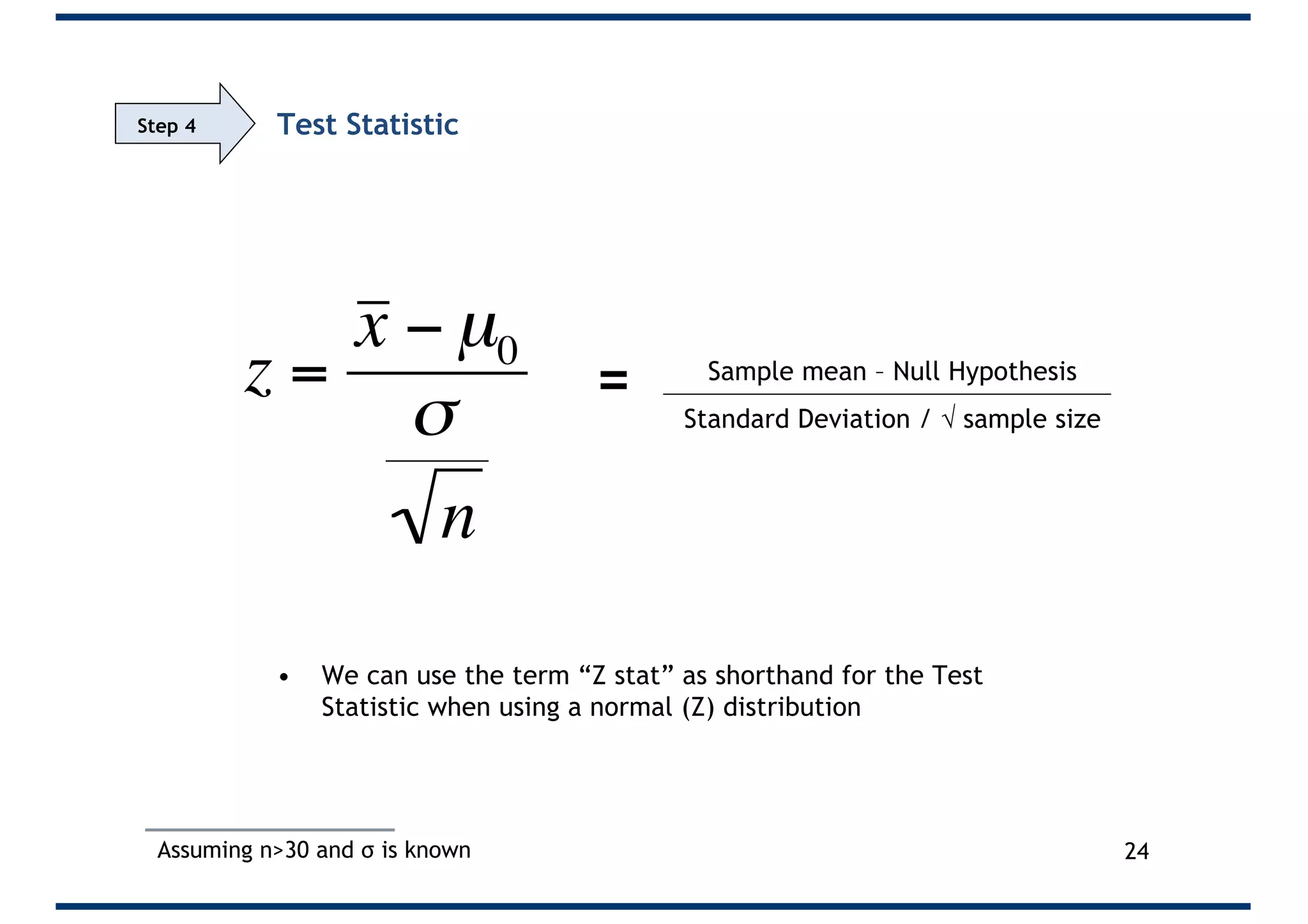
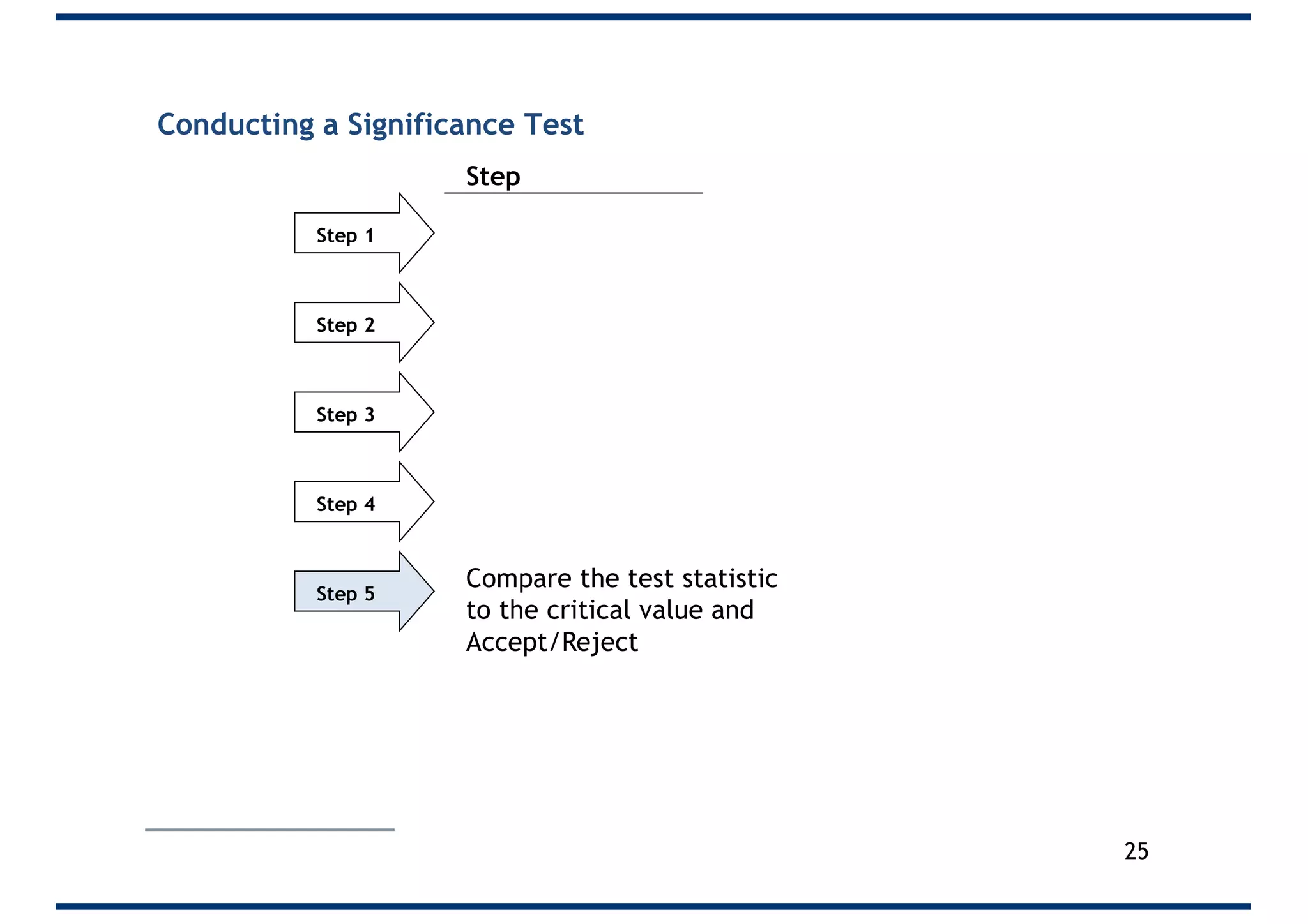
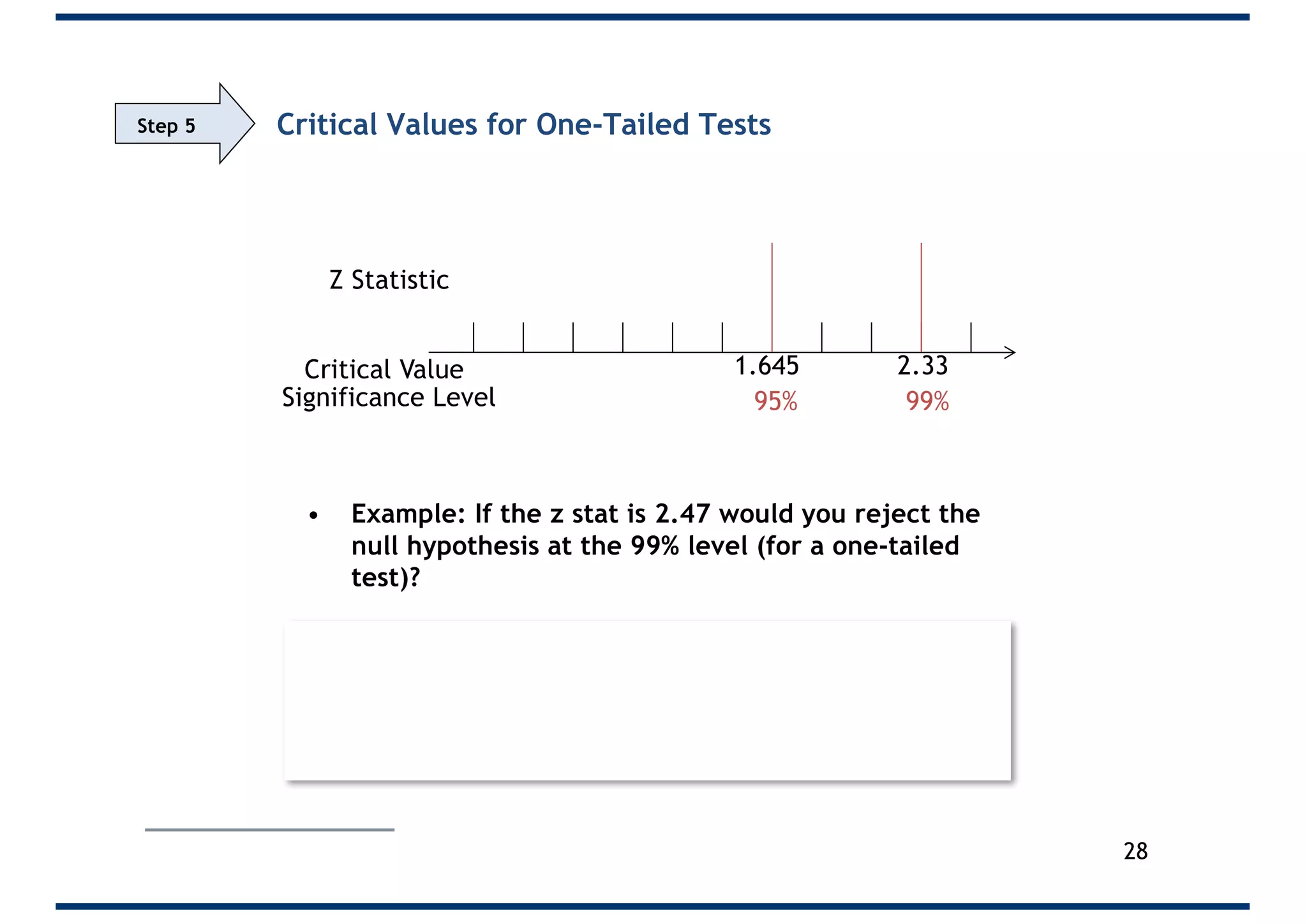
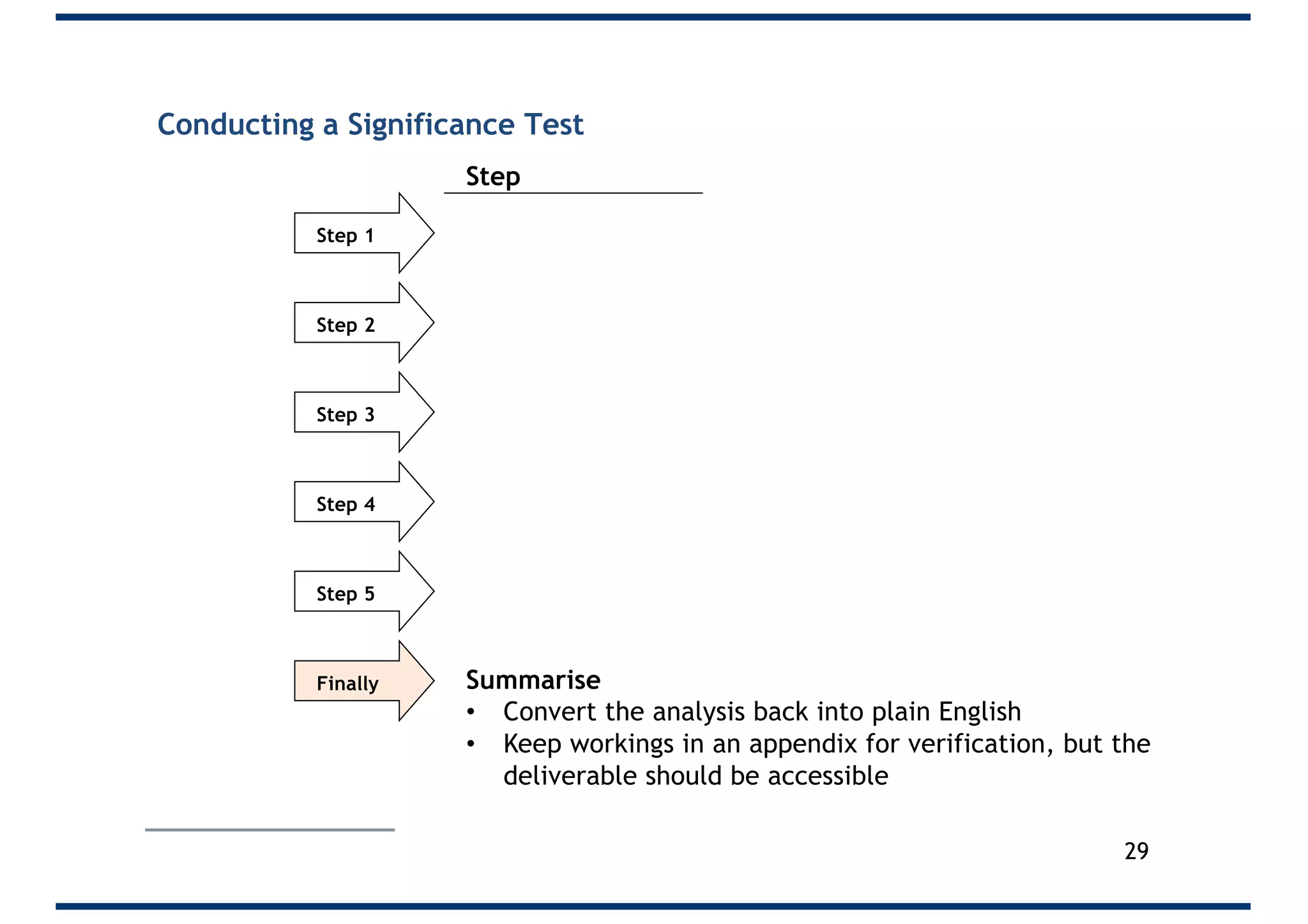
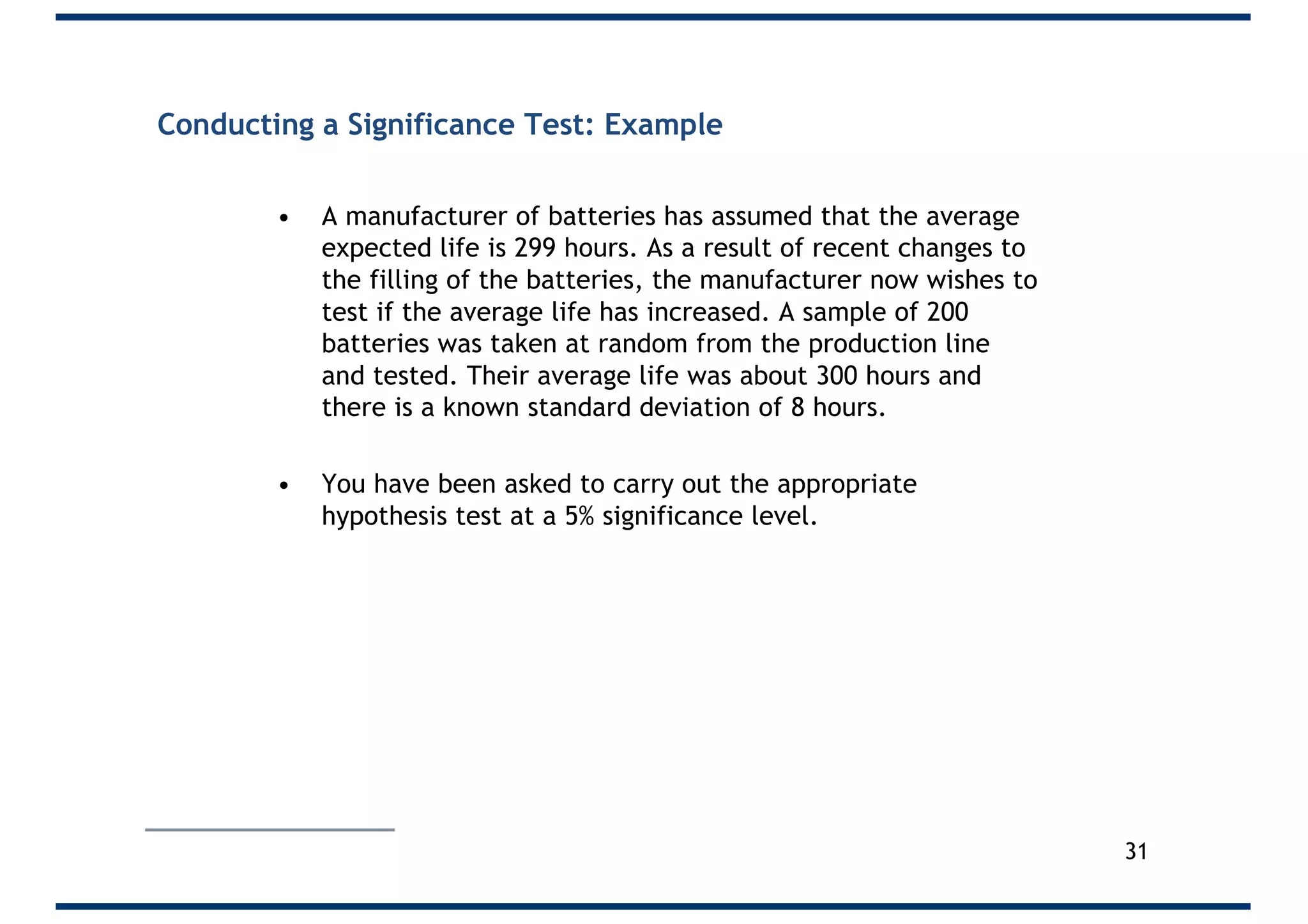
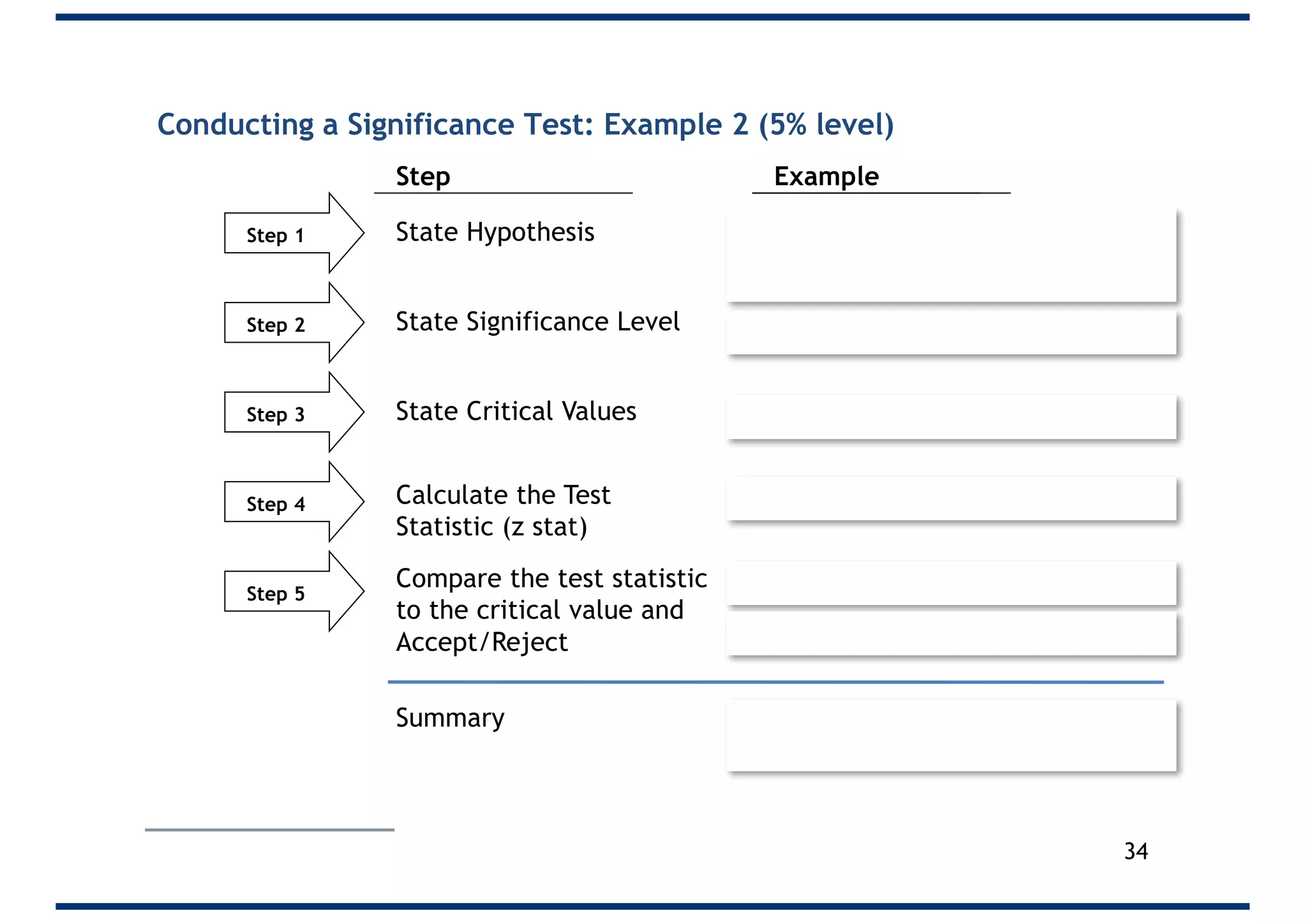
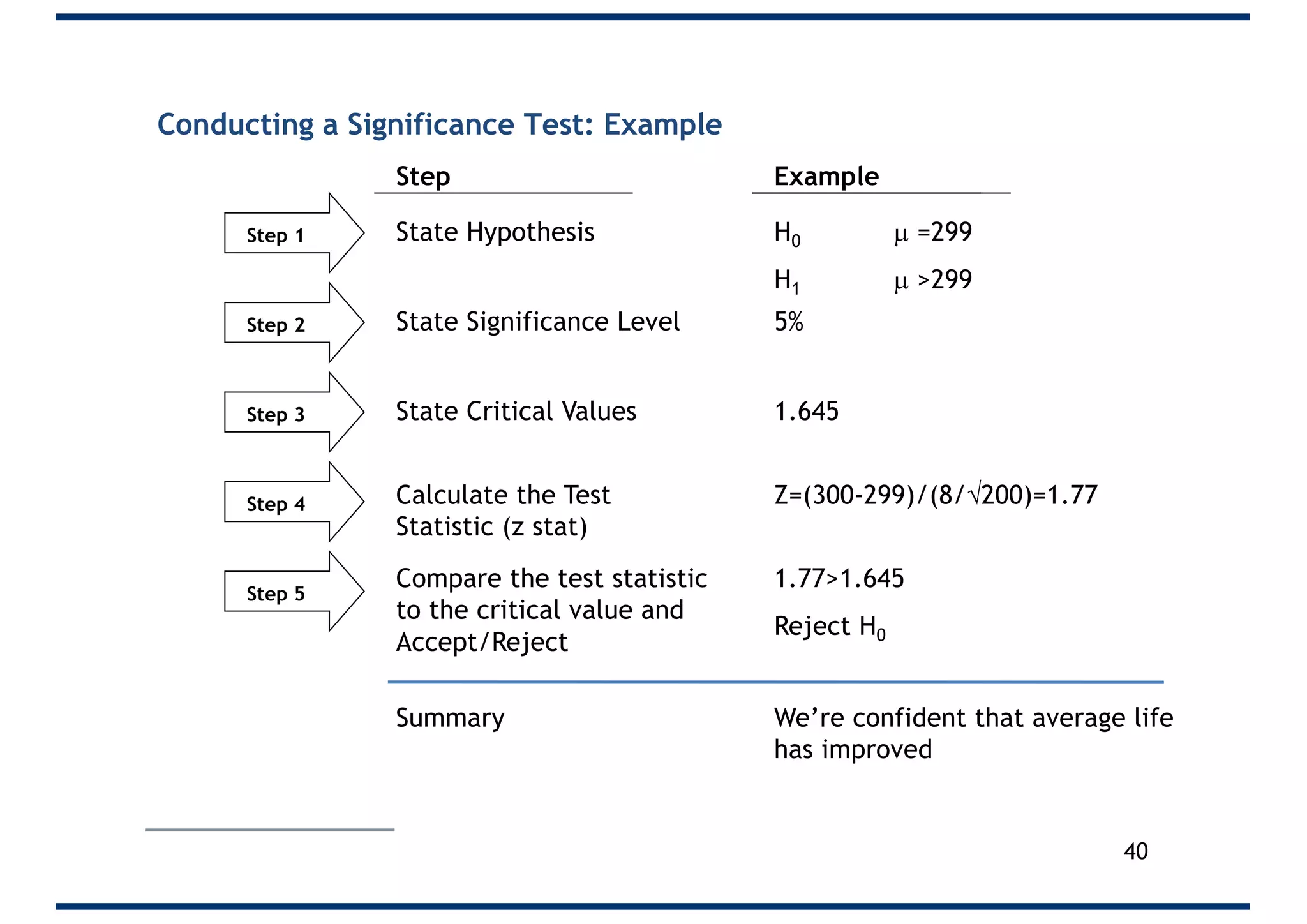
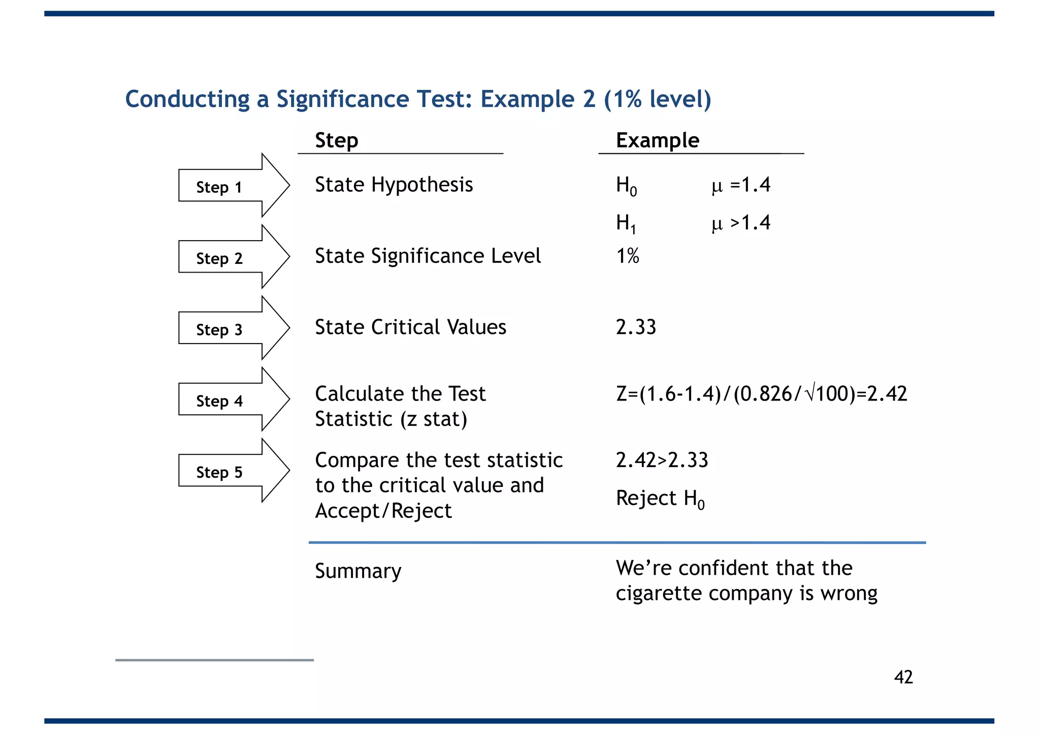
Statistical inference: Probability and DistributionEugene Yan Ziyou
This deck was used in the IDA facilitation of the John Hopkins' Data Science Specialization course for Statistical Inference. It covers the topics in week 1 (probability) and week 2 (distribution).
Statistical inference: Probability and DistributionEugene Yan Ziyou
This deck was used in the IDA facilitation of the John Hopkins' Data Science Specialization course for Statistical Inference. It covers the topics in week 1 (probability) and week 2 (distribution).
Random Variable
Discrete Probability Distribution
continuous Probability Distribution
Probability Mass Function
Probability Density Function
Expected value
variance
Binomial Distribution
poisson distribution
normal distribution
Quantitative Methods for Management_MBA_Bharathiar University probability dis...Victor Seelan
unit 3 probability distribution
Probability – definitions – addition and multiplication Rules (only statements) – simple business application problems – probability distribution – expected value concept – theoretical probability distributions – Binomial, Poison and Normal – Simple problems applied to business.
Probability distribution is a way to shape the sample data to make predictions and draw conclusions about an entire population because most improvement projects and scientific research studies are conducted with sample data rather than with data from an entire population. Probability distribution helps finding all the possible values a random variable can take between the minimum and maximum possible values
Theoretical probability distributions: Binomial, Poisson,
Normal and Exponential and also includes, discrete probability distributions, continuous probability distribution, random variables, sample problems
Testing of hypothesis - large sample testParag Shah
Different type of test which are used for large sample has been included in this presentation. Steps for each test and a case study is included for concept clarity and practice.
The Building Blocks of QuestDB, a Time Series Databasejavier ramirez
Talk Delivered at Valencia Codes Meetup 2024-06.
Traditionally, databases have treated timestamps just as another data type. However, when performing real-time analytics, timestamps should be first class citizens and we need rich time semantics to get the most out of our data. We also need to deal with ever growing datasets while keeping performant, which is as fun as it sounds.
It is no wonder time-series databases are now more popular than ever before. Join me in this session to learn about the internal architecture and building blocks of QuestDB, an open source time-series database designed for speed. We will also review a history of some of the changes we have gone over the past two years to deal with late and unordered data, non-blocking writes, read-replicas, or faster batch ingestion.
Quantitative Data AnalysisReliability Analysis (Cronbach Alpha) Common Method...2023240532
Quantitative data Analysis
Overview
Reliability Analysis (Cronbach Alpha)
Common Method Bias (Harman Single Factor Test)
Frequency Analysis (Demographic)
Descriptive Analysis
Adjusting OpenMP PageRank : SHORT REPORT / NOTESSubhajit Sahu
For massive graphs that fit in RAM, but not in GPU memory, it is possible to take
advantage of a shared memory system with multiple CPUs, each with multiple cores, to
accelerate pagerank computation. If the NUMA architecture of the system is properly taken
into account with good vertex partitioning, the speedup can be significant. To take steps in
this direction, experiments are conducted to implement pagerank in OpenMP using two
different approaches, uniform and hybrid. The uniform approach runs all primitives required
for pagerank in OpenMP mode (with multiple threads). On the other hand, the hybrid
approach runs certain primitives in sequential mode (i.e., sumAt, multiply).
1. A 5 Step Significance Test
Anthony J. Evans
Professor of Economics, ESCP Europe
www.anthonyjevans.com
(cc) Anthony J. Evans 2019 | http://creativecommons.org/licenses/by-nc-sa/3.0/
3. Null and Alternative Hypothesis
Definition
Status quo hypothesis,
starting assumption
Null hypothesis
Alternative
hypothesis
Other assumption, strong
belief, gut feeling
Examples
In the US system of justice, the guiding
principle is supposed to be that the
defendant is “presumed innocent until
proven guilty”. This claim of innocence
is a null hypothesis
The prosecution offers a competing
claim: the defendant is guilty. This is an
alternative to the null hypothesis of
innocence and we call the claim of guilt
an alternative hypothesis
H0
H1
3
Step 1
4. Null and Alternative Hypotheses
• H0: b=0; H1: b>0 One tailed
• H0: b=0; H1: b<0 One tailed
• H0: b=0; H1: b¹0 Two tailed
Remark:
Accepting the null hypothesis does not necessarily mean that we literally
believe that it is true. Sometimes it means that we do not have enough
evidence to reject it or that we are reserving judgement
4
Step 1
5. State Hypothesis
• The test is designed to assess the strength of the evidence
against H0
• H1 is the statement that we will accept if the evidence
enables us to reject H0
5
Step 1
6. State Hypothesis: Examples
What is the null hypothesis (H0) and what is the
alternative hypothesis (H1)?
Also, is it a one or two-sided test?
1. The mean area of the several thousand apartments in a
new development is advertised to be 1250 square feet. A
tenant group thinks that the apartments are smaller than
advertised. They hire an engineer to measure a sample of
the apartments to test their suspicion
2. Larry’s car averages 32 miles per gallon on the highway. He
now switches to a new motor oil that is advertised as
increasing gas mileage. After driving 3000 highway miles
with the new oil, he wants to determine if his gas mileage
has actually increased
6
Step 1
7. State Hypothesis: Examples (2)
1. The mean area of the several thousand apartments
in a new development is advertised to be 1250
square feet. A tenant group thinks that the
apartments are smaller than advertised. They hire
an engineer to measure a sample of the apartments
to test their suspicion
H0: µ = 1250
H1: µ < 1250 One sided
2. Larry’s car averages 32 miles per gallon on the
highway. He now switches to a new motor oil that is
advertised as increasing gas mileage. After driving
3000 highway miles with the new oil, he wants to
determine if his gas mileage has actually increased
H0: µ =32
H1: µ > 32 One Sided
7
Step 1
9. Significance Level
• Significance level has other names
– Probability value
– P-Value
– Alpha level
• We expect observations to have a random element, but
how confident can we be that the null hypothesis is wrong
because our theory is correct, instead of it just being
random error?
• There is a slight chance that an observation might come
from an extreme part of the distribution, but the chances
are very small
• So small, in fact, that we can conclude that it’s not a
random error, but the predicted result of your theory
• If there’s a large difference between the sample evidence
and the null hypothesis, we conclude that the alternative
hypothesis is more likely to be correct
9
Step 2
10. Significance Level
• To make this judgement we decide on critical values,
which define the points at which the probability of the
null hypothesis being true is at a small, predetermined
level
• Typical significance levels are 0.1 (10%), 0.05 (5%), and
0.01 (1%)
– These values correspond to the probability of observing
such an extreme value by chance
• We can divide up the Normal distribution diagram into
sections, see whether the z-value falls into a particular
section, and thus reject or accept the null hypothesis
• Generally, the smaller the significance level, the more
people there are who would be willing to say that the
alternative hypothesis beats the null hypothesis
• The p-value is the lowest level of significance at which
we can reject the null hypothesis
10
Step 2
12. Two sided test
One sided tests
a / 2 a / 21 - a
– z + z
Do Not Reject H0
Reject H0Reject H0
a
1 - a
– z
Do Not Reject H0Reject H0
a1 - a
+ z
Do Not Reject H0
0
Reject H0
One vs. Two Sided TestsStep 3
13. 5% Significance Levels for One-Tailed Tests
x
Reject
Do notreject
Rejection Regions
Critical Value
5%
95%
13
Step 3
14. 1% Significance Levels for One-Tailed Tests
x
Reject
Do notreject
Rejection Regions
Critical Value
1%
99%
14
Step 3
15. 5% Significance Levels for Two-Tailed Tests
x
RejectReject
Do notreject
Rejection Regions
Critical ValueCritical Value
2.5%2.5%
95%
15
Step 3
16. 1% Significance Levels for Two-Tailed Tests
x
RejectReject
Do notreject
Rejection Regions
Critical ValueCritical Value
0.5%0.5%
99%
16
Step 3
17. Significance Level à Critical Value
• For each significance level (e.g. 5%), we can use a Normal
probability table to ascertain the relevant critical value
(given as Z)
• Note: I’m showing you how to go from significance level to
critical value but we could do it in both directions
17
Step 3
18. Standard Normal Cumulative Probability Table
• Let’s say I want to find the critical value (Z) that is
associated with a 5% confidence level, (one-tailed)
18
Step 3
19. Standard Normal Cumulative Probability Table
• Let’s say I want to find the critical value (Z) that is
associated with a 5% confidence level, (one-tailed)
• 95% of the population will be below the critical
value
z =
1.645
Looking
for 0.05
19
Step 3
20. Standard Normal Cumulative Probability Table
z =
2.33
Looking
for 0.01
• Let’s say I want to find the critical value (Z) that is
associated with a 1% confidence level, (one-tailed)
• 99% of the population will be below the critical
value
20
Step 3
21. Standard Normal Cumulative Probability Table
• Let’s say I want to find the critical value (Z) that is
associated with a 5% confidence level, (two-tailed)
• 97.5% of the population will be below the critical
value
z =
1.96
Looking
for 0.025
21
Step 3
22. The relationship between confidence level (C), p value (P)
and Z for 1 and 2 tailed tests
At the 95% level, there is a 2.5% chance that we would see this result (or something even more extreme), if the
sample mean really is the population mean. Therefore a small p value tells us one of two things:
• Our observation is so extreme we can reject the hypothesis that the sample belongs to the overall population
• The hypothetical event is very unlikely to come given from the sample we have
Level of
confidence
C P2 Z2 Z1
A little 68% 0.16 1 -
Fairly 90% 0.05 1.645 1.282
Very 95% 0.025 1.96 1.645
Very 95.4% 0.023 2 -
Highly 99% 0.005 2.576 2.33
Extremely 99.7% 0.0015 3 -
22
Step 3
23. Conducting a Significance Test
Step 1
Step 2
Step 3
Step 4
Step 5
Calculate the Test
Statistic (z)
Step
23
24. Test Statistic
• We can use the term “Z stat” as shorthand for the Test
Statistic when using a normal (Z) distribution
24
Sample mean – Null Hypothesis
Standard Deviation / Ö sample size
Assuming n>30 and σ is known
=
Step 4
z =
x − µ0
σ
n
25. Conducting a Significance Test
Step 1
Step 2
Step 3
Step 4
Step 5
Compare the test statistic
to the critical value and
Accept/Reject
Step
25
26. Critical Value (i.e. Probability Value) and Test Statistic
• A critical value is the value that a test statistic
must exceed in order for the null hypothesis to be
rejected.
• It should be noted that the all-or-none rejection of a
null hypothesis is not recommended
26
Step 5
27. Critical Values for One-Tailed Tests
Critical Value 1.645 2.33
Significance Level 95% 99%
Z Statistic
• Example: If the z stat is 1.83 would you reject the
null hypothesis at the 95% level (for a one-tailed
test)?
• Yes, since
1.83 > 1.645
z > critical value
So REJECT at the 95% level
1.83
27
Step 5
28. Critical Values for One-Tailed Tests
Critical Value 1.645 2.33
Significance Level 95% 99%
Z Statistic
• Example: If the z stat is 2.47 would you reject the
null hypothesis at the 99% level (for a one-tailed
test)?
• Yes, since
2.47 > 2.33
z > critical value
So REJECT at the 99% level
2.47
28
Step 5
29. Conducting a Significance Test
Step 1
Step 2
Step 3
Step 4
Step 5
Finally Summarise
• Convert the analysis back into plain English
• Keep workings in an appendix for verification, but the
deliverable should be accessible
Step
29
30. Conducting a Significance Test: Recap
Step 1
Step 2
Step 3
Step 4
Step 5
Step
State Hypothesis
State Significance Level
State Critical Values
Calculate the Test
Statistic (z)
30
Compare the test statistic
to the critical value and
Accept/Reject
31. Conducting a Significance Test: Example
• A manufacturer of batteries has assumed that the average
expected life is 299 hours. As a result of recent changes to
the filling of the batteries, the manufacturer now wishes to
test if the average life has increased. A sample of 200
batteries was taken at random from the production line
and tested. Their average life was about 300 hours and
there is a known standard deviation of 8 hours.
• You have been asked to carry out the appropriate
hypothesis test at a 5% significance level.
31
32. Conducting a Significance Test: Example
Step 1
Step 2
Step 3
Step 4
Step 5
Summary
Step Example
State Hypothesis
State Significance Level
State Critical Values
Calculate the Test
Statistic (z stat)
Compare the test statistic
to the critical value and
Accept/Reject
We’re confident that average life
has improved
H0 µ =299
H1 µ >299
5%
1.645
Z=(300-299)/(8/Ö200)=1.77
1.77>1.645
Reject H0
32
33. Conducting a Significance Test: Example 2
• A particular brand of cigarettes advertises that their
cigarettes contain 1.4 milligrams of nicotine.
• An anti-smoking group perform a survey of 100 cigarettes,
and find a sample mean of 1.6 milligrams
• Assume that the standard deviation is 0.826
• The group want to claim that there’s more nicotine in their
cigarettes than the company admit
• Is the result significant at the 5% level?
• Is the results significant at the 1% level?
33
34. Conducting a Significance Test: Example 2 (5% level)
Step 1
Step 2
Step 3
Step 4
Step 5
Step Example
State Hypothesis
State Significance Level
State Critical Values
Calculate the Test
Statistic (z stat)
Compare the test statistic
to the critical value and
Accept/Reject
We’re confident that the
cigarette company is wrong
H0 µ =1.4
H1 µ >1.4
5%
1.645
Z=(1.6-1.4)/(0.826/Ö100)=2.42
2.42>1.645
Reject H0
Summary
34
35. Conducting a Significance Test: Example 2 (1% level)
Step 1
Step 2
Step 3
Step 4
Step 5
Step Example
State Hypothesis
State Significance Level
State Critical Values
Calculate the Test
Statistic (z stat)
H0 µ =1.4
H1 µ >1.4
1%
2.33
Z=(1.6-1.4)/(0.826/Ö100)=2.42
2.42>2.33
Reject H0
We’re confident that the
cigarette company is wrong
Summary
35
Compare the test statistic
to the critical value and
Accept/Reject
37. State Hypothesis: Examples (2)
1. The mean area of the several thousand apartments
in a new development is advertised to be 1250
square feet. A tenant group thinks that the
apartments are smaller than advertised. They hire
an engineer to measure a sample of the apartments
to test their suspicion
H0: µ = 1250
H1: µ < 1250 One sided
2. Larry’s car averages 32 miles per gallon on the
highway. He now switches to a new motor oil that is
advertised as increasing gas mileage. After driving
3000 highway miles with the new oil, he wants to
determine if his gas mileage has actually increased
H0: µ =32
H1: µ > 32 One Sided
37
Step 1
38. Critical Values for One-Tailed Tests
Critical Value 1.645 2.33
Significance Level 95% 99%
Z Statistic
• Example: If the z stat is 1.83 would you reject the
null hypothesis at the 95% level (for a one-tailed
test)?
• Yes, since
1.83 > 1.645
z > critical value
So REJECT at the 95% level
1.83
38
Step 5
39. Critical Values for One-Tailed Tests
Critical Value 1.645 2.33
Significance Level 95% 99%
Z Statistic
• Example: If the z stat is 2.47 would you reject the
null hypothesis at the 99% level (for a one-tailed
test)?
• Yes, since
2.47 > 2.33
z > critical value
So REJECT at the 99% level
2.47
39
Step 5
40. Conducting a Significance Test: Example
Step 1
Step 2
Step 3
Step 4
Step 5
Summary
Step Example
State Hypothesis
State Significance Level
State Critical Values
Calculate the Test
Statistic (z stat)
Compare the test statistic
to the critical value and
Accept/Reject
We’re confident that average life
has improved
H0 µ =299
H1 µ >299
5%
1.645
Z=(300-299)/(8/Ö200)=1.77
1.77>1.645
Reject H0
40
41. Conducting a Significance Test: Example 2 (5% level)
Step 1
Step 2
Step 3
Step 4
Step 5
Step Example
State Hypothesis
State Significance Level
State Critical Values
Calculate the Test
Statistic (z stat)
Compare the test statistic
to the critical value and
Accept/Reject
We’re confident that the
cigarette company is wrong
H0 µ =1.4
H1 µ >1.4
5%
1.645
Z=(1.6-1.4)/(0.826/Ö100)=2.42
2.42>1.645
Reject H0
Summary
41
42. Conducting a Significance Test: Example 2 (1% level)
Step 1
Step 2
Step 3
Step 4
Step 5
Step Example
State Hypothesis
State Significance Level
State Critical Values
Calculate the Test
Statistic (z stat)
H0 µ =1.4
H1 µ >1.4
1%
2.33
Z=(1.6-1.4)/(0.826/Ö100)=2.42
2.42>2.33
Reject H0
We’re confident that the
cigarette company is wrong
Summary
42
Compare the test statistic
to the critical value and
Accept/Reject
43. • This presentation forms part of a free, online course
on analytics
• http://econ.anthonyjevans.com/courses/analytics/
43