Professor Evans studies taxi journey prices from Hertfordshire to Heathrow using receipts from 100 journeys to infer the population average price. He calculates the sample mean as €32.36, finds a 95% confidence interval for the population average between €30.93 and €33.79, and concludes there is statistical significance that the true average is above €30.85. This analysis raises additional questions about distribution assumptions and pricing models.

1. Taxi for Professor Evans
An introduction to inferential statistics
Anthony J. Evans
Professor of Economics, ESCP Europe
www.anthonyjevans.com
(cc) Anthony J. Evans 2019 | http://creativecommons.org/licenses/by-nc-sa/3.0/

2. Introduction
Professor Evans wants to learn more about the prices of taxi
journeys from his home in Hertfordshire to Heathrow airport.
He contacts the local taxi company, who give him the receipts
from 100 similar journeys (given in €). His aim is to use this
sample to make an inference about the market as a whole.
There are three main questions he wishes to understand:
1. What is his best estimate of the population average (µ)?
2. Within what range would he be reasonably confident of the
population average (µ) being?
3. Is the population average (µ) likely to be above €30.85?
2Download data set from: http://econ.anthonyjevans.com/cases
𝑛 = 100
𝑥̅ = 32.36
𝑠 = 7.13

3. 1. What is his best estimate of the population average (µ)?
• The sample mean (x’) serves as a suitable best estimate of
the population average (µ), provided the population
distribution is:
– Symmetric
– No extreme outliers
• The mean is a measure of location
• We also need to understand a measure of dispersion
3
𝑥̅ = 32.36
𝑥̅ =
Σ𝑥.
𝑛

4. Statistical estimation - standard deviation
4S is a sample standard deviation, which is an estimate of σ.
Dividing by n-1 is Bessel's correction to compensate for the fact that it’s a biased estimate
Total 5028.26
Total/(n-1) 50.79
SQRT 7.13
i Xi Xi - X' (Xi - X')2
1 28.80 -3.56 12.66
2 24.00 -8.36 69.86
3 22.00 -10.36 107.29
4 42.00 9.64 92.97
5 34.00 1.64 2.70
6 47.60 15.24 232.32
7 50.40 18.04 325.51
8 39.20 6.84 46.81
9 40.60 8.24 67.93
10 51.80 19.44 377.99
… … … …
90 27.20 -5.16 26.60
91 28.80 -3.56 12.66
92 22.40 -9.96 99.16
93 23.20 -9.16 83.87
94 29.60 -2.76 7.61
95 24.00 -8.36 69.86
96 25.60 -6.76 45.67
97 25.60 -6.76 45.67
98 28.00 -4.36 18.99
99 28.80 -3.56 12.66
100 28.00 -4.36 18.99
𝑠 =
Σ 𝑥. − 𝑥̅ 0
𝑛 − 1

5. 68% of values are within 1σ of µ
99.7% of values are within 3σ of µ
95% of values are within 2σ of µ
The normal distribution and the 68-95-99.7 rule
5Note: we can use this to say that 95% of the sample distribution will be 2 standard deviation (s) either side
of the sample mean (x’)

6. Standard error
• How precise are our estimates? The standard error
(SE) of a value is the estimated standard deviation of
the process by which it was generated, adjusted for
the sample size
• If a distribution is normal, 95% of observations are
within 2 standard deviations of the mean (95% are
x’±2σ)
• For a sample, 95% of the sample means are within 2
standard errors of the population mean (µ)
• Ideally you want a low standard error, i.e.
– A low sample standard deviation (s)
– A large sample size (n)
6For example, if n=200 then SE would fall to 7.13/(SQRT200) = 0.50
𝑆𝐸 =
𝑠
𝑛

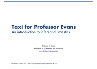
7. 2. Within what range would he be reasonably confident of the
population average (µ) being?
• 68% confidence interval
– 1 SE from the mean =
• 95% confidence interval
– 2 SE from the mean =
• 99.7% confidence interval
– 3 SE from the mean =
7A 95% confidence interval means “if you sampled many different populations and for each sample
constructed a 95% confidence interval, then 95% of the time the true population mean would lie within the
corresponding interval”
𝑥̅ = 32.36
1×
7.13
100
2×
7.13
100
3×
7.13
100
= ±0.71
= ±1.43
= ±2.14
= [31.65,33.07]
= [30.93,33.79]
= [30.22,34.50]

8. Aside: Why are 95% of values within 2SE of the mean?
8

9. Aside: Why are 95% of values within 2SE of the mean?
9
2
0.02275
0.02275
- 2
0.954

10. Summary
10
33.0730.93 31.65 33.7930.22 34.5032.36
−3𝑆𝐸 −2𝑆𝐸 −1𝑆𝐸 1𝑆𝐸 2𝑆𝐸 3𝑆𝐸𝑥̅

11. Confidence Intervals
• There is a probability, C that the interval given below
contains µ
• z* is the value on the standard normal curve with area C
between –z* and z*
11For simplicity we are assuming that σ is known
𝑥̅ ± 𝑧×
𝜎
𝑛

12. Statistical significance
• Let’s say we are especially interested to know whether the
true average is likely to be above €30.85
– For example, this is amount that can be claimed on
expenses
• The sample mean suggests this is the case, since €32.36 >
€30.85, but how likely is it that the population mean (µ) is
as well?
• The sample outcome is statistically significant if it falls
outside of our confidence interval
• A sample result is statistically significant at the 2.5% level
if the critical value falls outside a 95% confidence interval
12

13. 3. Is the population average (µ) likely to be above €30.85?
13
95%
We are only 2.5%
confident that the
true population mean
would be within this
region
30.93 33.7932.36

14. Significance testing
• Let’s assume that the population mean is indeed €30.85
• What is the probability of finding a sample mean of €32.36?
• Step A: Calculate how many standard errors the sample
mean is from our hypothesis about the population mean
• Step B: Determine how likely this would be
14This is reversing the process we used when constructing a confidence interval. Then, we established a 95%
level of confidence (z=2) and calculated the corresponding vales. Now, we want to find the level of
confidence associated with a specific value

15. Step A: Calculate the z score
15For simplicity take the absolute value of Z
𝑧 =
𝑥̅ − 𝜇
𝑆𝐸
=
32.36 − 30.85
7.13
100
@
= 2.12

16. 16
Step B: Determine how likely this would be

17. There is only a 1.7% chance of observing a sample mean this high
17
2.12
0.017
30.85 32.36

18. This is statistically significant at the 95% level
18
2.12
1.645
0.05
There is enough
evidence to reject the
assumption that this is
just a freak sample

19. This is not statistically significant at the 99% level
19
2.33
0.01
2.12
There is not enough
evidence to reject the
assumption that this is
just a freak sample

20. Solutions
1. What is his best estimate of the population average (µ)?
– €32.36
2. Within what range would he be reasonably confident of the
population average (µ) being?
– Between €30.93 and €33.79
3. Is the population average (µ) likely to be above €30.85?
– Yes, our sample provides a statistically significant
estimate that the true average is above €30.85 (at
the 95% level)
20

21. Discussion questions
• What if it isn’t normally distributed?
• What if the sample isn’t representative of the typical consumer?
– Maybe the receipts relate to different journeys
• What are the costs of a variable pricing model?
– Why don’t they charge a flat rate?
• Wouldn’t the price from the airport be more than the price to the
airport?
– Are these two different distributions?
• What if the underlying distribution changes?
– A new tax on petrol
– A train/tube strike that meant taxis were the only way to get
to the airport
• Even if it is statistically significant, does it have oomph?
21

22. The relationship between confidence level (C), p value (P) and Z for 1
and 2 tailed tests
At the 95% level, there is a 2.5% chance that we would see this result (or something even more extreme), if the
sample mean really is the population mean. Therefore a small p value tells us one of two things:
• Our observation is so extreme we can reject the hypothesis that the sample belongs to the overall population
• The hypothetical event is very unlikely to come given from the sample we have
Level of
confidence
C P2 Z2 Z1
A little 68% 0.16 1 -
Fairly 90% 0.05 1.645 1.282
Very 95% 0.025 1.96 1.645
Very 95.4% 0.023 2 -
Highly 99% 0.005 2.576 2.33
Extremely 99.7% 0.0015 3 -
22

23. The normal distribution
23

24. Other distributions
• Binomial
– Used when there are two possible outcomes and are
independent events
• Poisson
– Used to find the probability of a given event occurring
in a fixed interval of time
• T-distribution
– Used for small (n<30) sample sizes
24