Modern_Distribution_Presentation.pptx

1. BINOMIAL ,POISSON AND
NORMAL DISTRIBUTION ..
Muhammad Awais

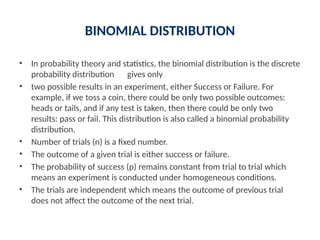
2. BINOMIAL DISTRIBUTION
• In probability theory and statistics, the binomial distribution is the discrete
probability distribution gives only
• two possible results in an experiment, either Success or Failure. For
example, if we toss a coin, there could be only two possible outcomes:
heads or tails, and if any test is taken, then there could be only two
results: pass or fail. This distribution is also called a binomial probability
distribution.
• Number of trials (n) is a fixed number.
• The outcome of a given trial is either success or failure.
• The probability of success (p) remains constant from trial to trial which
means an experiment is conducted under homogeneous conditions.
• The trials are independent which means the outcome of previous trial
does not affect the outcome of the next trial.

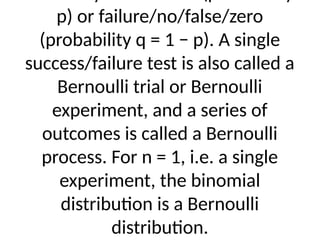
3. p) or failure/no/false/zero
(probability q = 1 − p). A single
success/failure test is also called a
Bernoulli trial or Bernoulli
experiment, and a series of
outcomes is called a Bernoulli
process. For n = 1, i.e. a single
experiment, the binomial
distribution is a Bernoulli
distribution.

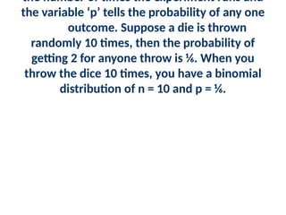
4. the number of times the experiment runs and
the variable ‘p’ tells the probability of any one
outcome. Suppose a die is thrown
randomly 10 times, then the probability of
getting 2 for anyone throw is ⅙. When you
throw the dice 10 times, you have a binomial
distribution of n = 10 and p = ⅙.

5. FORMULA

6. p = Probability of Success in a
single experiment
q = Probability of Failure in a single
experiment = 1 – p
The binomial distribution formula
can also be written in the form of
n-Bernoulli trials, where nCx =
n!/x!(n-x)!. Hence,
P(x:n,p) = n!/[x!(n-x)!].px.(q)n-x

7. Binomial Distribution
• Mean and Variance
• For a binomial distribution, the mean, variance and standard deviation for
the given number of success are represented using the formulas
• Mean, μ = np
• Variance, σ2 = npq
• Standard Deviation σ= √(npq)
• Where p is the probability of success
• q is the probability of failure, where q = 1-p

8. PROPERTIES OF BINOMIAL DISTRIBUTION
• The properties of the binomial distribution are:
• There are two possible outcomes: true or false, success or failure, yes or
no.
• There is ‘n’ number of independent trials or a fixed number of n times
repeated trials.
• The probability of success or failure remains the same for each trial.
• Only the number of success is calculated out of n independent trials.
• Every trial is an independent trial, which means the outcome of one trial
does not affect the outcome of another trial.

9. It is a p.m.f.(probability mass function).
• The parameters of Binomial Distribution are ’n’ and ‘p’ where, n - number
of trials and p - probability of
• success.
• Mean of Binomial Distribution = np
• Variance of Binomial Distribution = npq (here q=1-p)
• Mode of Binomial Distribution is integral part of (n+1)p, if (n+1)p is not an
integer. But, if (n+1)p is an integer, then the distribution has two modal
values, (n+1)p and [(n+1)p] - 1.
• q- probability of failure, q < 1, hence, npq < np. Thus, Variance is less than
Mean.
• If p=q=1/2, then the distribution is symmetric about median and if p is not
equal to q, then it is skewed distribution.
• Additive property of Binomial Distribution : If X and Y are independent
variables such that X follows Binomial Distribution with (n1, p) and Y
follows Binomial Distribution with (n2, p), then (X+Y) follows Binomial
Distribution with (n1+n2, p).

10. What are the criteria for the binomial
distribution
• The number of trials should be fixed.
• Each trial should be independent.
• The probability of success is exactly the same from one trial to the
other trial.

11. in an election.
The number of successful sales
calls.
The number of male/female
workers in a company
So, as we have the basis let’s see
some binominal distribution
examples, problems, and solutions
from real life.

12. Binomial Distribution Vs NormalDistribution
• Binomial Distribution Vs Normal Distribution
• The main difference between the binomial distribution and the
normal distribution is that binomial distribution is discrete, whereas the
normal distribution is continuous. It means that the binomial distribution
has a finite amount of events, whereas the normal distribution has an
infinite number of events. In case, if the sample size for the
binomial distribution is very large, then the distribution curve for the
binomial distribution is similar to the normal distribution curve
• •

13. Poission Distribution

14. Poisson Distribution
• Poisson distribution is a theoretical discrete probability and is also known
as the Poisson distribution probability mass function. It is used to
find the probability of an independent event that is occurring in a fixed
interval of time and has a constant mean rate. The Poisson
distribution probability mass function can also be used in other fixed
intervals such as volume, area, distance, etc. A Poisson random variable
will relatively describe a phenomenon if there are few successes over
many trials. The Poisson distribution is used as a limiting case of the
binomial distribution when the trials are large indefinitely. If a Poisson
distribution models the same binomial phenomenon, λ is replaced
by np. Poisson distribution is named after the French
mathematician Denis Poisson

15. Poisson distribution
• Poisson distribution definition is used to model a discrete probability
of an event where independent events are occurring in a fixed
interval of time and have a known constant mean rate. In other
words, Poisson distribution is used to estimate how many times an
event is likely to occur within the given period of time. λ is the
Poisson rate parameter that indicates the expected value of the average
number of events in the fixed time interval. Poisson distribution has wide
use in the fields of business as well as in biology

16. Example :
• Let us try and understand this with an example, customer care
center receives 100 calls per hour, 8 hours a day. As we can see
that the calls are independent of each other. The probability of the
number of calls per minute has a Poisson probability distribution. There
can be any number of calls per minute irrespective of the number of
calls received in the previous minute. Below is the curve of the
probabilities for a fixed value of λ of a function following Poisson
distribution:

17. FORMULA
• Poisson distribution formula is used to find the probability of an
event that happens independently, discretely over a fixed time
period, when the mean rate of occurrence is constant over time. The
Poisson distribution formula is applied when there is a large number of
possible outcomes. For a random discrete variable X that follows the
Poisson distribution, and λ is the average rate of value, then the
probability of x is given by:
• f(x) = P(X=x) = (e-λ λx )/x!
• •

18. For Poisson distribution, which has
λ as the average rate, for a fixed
interval of time, then the mean of
the Poisson distribution and the
value of variance will be the same.
So for X following Poisson
distribution, we can say that λ is
the mean as well as the variance of
the distribution.

19. λ > 0
Properties of Poisson Distribution
The Poisson distribution is
applicable in events that have a
large number of rare and
independent
possible events

20. Important Notes
• The formula for Poisson distribution is f(x) = P(X=x) = (e-λ λx )/x!.
• For the Poisson distribution, λ is always greater than 0.
• For Poisson distribution, the mean and the variance of the distribution
are equal.

21. PROPERTIES
• The events are independent.
• The average number of successes in the given period of time alone can
occur. No two events can occur at the same time.
• The Poisson distribution is limited when the number of trials n is
indefinitely large.
• mean = variance = λ
• np = λ is finite, where λ is constant.
• The standard deviation is always equal to the square root of the mean μ.
• The exact probability that the random variable X with mean μ =a is given
by P(X= a) = μa / a! e -μ
• If the mean is large, then the Poisson distribution is approximately a
normal distribution

22. Poisson distribution table
• Similar to the binomial distribution, we can have a Poisson distribution
table which will help us to quickly find the probability mass
function of an event that follows the Poisson distribution. The Poisson
distribution table shows different values of Poisson distribution for
various values of λ, where λ>0. Here in the table given below, we can
see that, for P(X =0) and λ = 0.5, the value of the probability mass
function is 0.6065 or 60.65%.

24. NORMAL DISTRIBUTION

26. What are the properties of the normal
distribution?
• The normal distribution is a continuous probability distribution that is
symmetrical on both sides of the mean, so the right side of the centre is a
mirror image of the left side.
• The area under the normal distribution curve represents probability and
• the total area under the curve sums to one.
• Most of the continuous data values in a normal distribution tend to cluster
around the mean, and the further a value is from the mean, the less likely
it is to occur. The tails are asymptotic, which means that they approach
but never quite meet the horizon (i.e. x-axis).
• For a perfectly normal distribution the mean, median and mode will be
• the same value, visually represented by the peak of the curve

27. curve because the graph of its probability
density looks like a bell. It is also known as
called Gaussian distribution, after the German
mathematician Carl Gauss who first described
it.

28. What is the difference between a normal
distribution and a standard normal
distribution?
• A normal distribution is determined by two parameters the mean and the
variance. A normal distribution with a
• mean of 0 and a standard deviation of 1 is called a standard normal
distribution.

29. Why is the normal distribution important?
• The bell-shaped curve is a common feature of nature and psychology
• The normal distribution is the most important probability distribution in
statistics because many continuous data in nature and psychology displays
this bell-shaped curve when compiled and graphed.
• For example, if we randomly sampled 100 individuals we would expect to
see a normal distribution frequency curve for many continuous variables,
such as IQ, height, weight and blood pressure.

30. psychologists require
data to be normally distributed. If
the data does not resemble a bell
curve researchers may have to use
a less powerful type of statistical
test, called non-parametric
statistics.
• Converting the raw scores of a normal distribution to z-scores
• We can standardized the values (raw scores) of a normal distribution by
• converting them into z-scores.
• This procedure allows researchers to determine the proportion of the
values that fall within a specified number of standard deviations from the
mean (i.e. calculate the empirical rule).

31. What is the empirical rule formula?
• The empirical rule in statistics allows researchers to determine the
proportion of values that fall within certain distances from the
mean. The empirical rule is often referred to as the three-sigma
rule or the 68-95-99.7 rule.

33. researchers to calculate the
probability of randomly obtaining a
score from a normal distribution.
68% of data falls within the first
standard deviation from the mean.
This means there is a 68%
probability of randomly selecting a
score between -1 and +1 standard
deviations from the mean.

34. 95% of the values fall within two standard
deviations from the mean. This means there is
a 95% probability of randomly selecting a score
between -2 and +2 standard deviations from
the mean.
• 99.7% of data will fall within three standard deviations from the mean.
This means there is a 99.7% probability of randomly selecting a score
between -3 and +3 standard deviations from the mean.