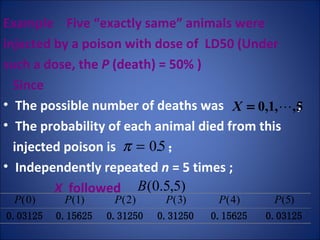
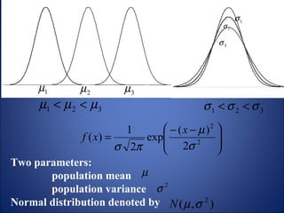
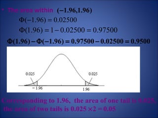
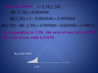
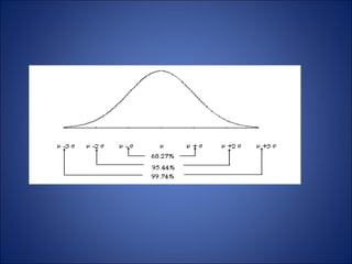
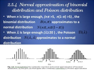
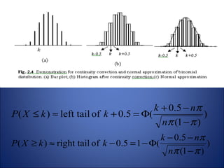
Chapter-2
Chapter 2 Probability and Distribution
Regular statement in statistics Two parts :  Conclusion  Probability that  the conclusion is true
2.1  Explanation of Probability and Related Concepts 2.1.1 Probability Flipping a die ( 骰子 ) Possible outcome:  1, 2, …, 6  Probability of “1”=  1/6 Color blindness test Possible outcome: normal, abnormal Probabilities of “abnormal”= ?  ---- Unknown! Survey:  Randomly selected  n  students,  if  m  of them are color blinders, then probability of abnormal  
In general,  Events:  the possible outcomes  ,… Probability  of the event  E  :  P ( E ).  ---- between 0 and 1  Conditional probability : Under the condition that  appears, the  probability of the event  For example,  P ( nasopharyngeal carcinoma∣ EB virus +)
2.1.2  Odds   Complementary event : If there are only two possible events and they are exclusive, denoted  with  and  , then  Odds of event E :  Question : Football game between teams A and B, If P(A win)=0.8,  then P(B win)=?  Odds (A win)=?  Odds (B win)=?
Eg.  If the incidence rates of influenza in classes A, B and C  are 60% , 50% and 40% then   Odds: To measure risk Odds ratio: To compare risks
2.1.3  Bayes ’  formula Smoking ( A )   -> Lung cancer ( B ) ?  Randomly divide the subjects into two groups; Invite one group to smoke and forbid another;  Follow up year by year to obtain the number of  the subjects “with lung cancer” …… Unfortunately, it is morally infeasible.  Then how?
To find  by Bayes’ formula Example 2.1
Conclusion: The risk of lung cancer for smoker is 5 times as much as that for ordinary people.
2.3 Binomial Distribution P ( white ball)=0.8 P (  yellow ball )=0.2 
In general, if : the  probability  of an event appearing in a trial  n   : times of  independently repeated  trials X   : random variable,  total times  of appearing such an event, then the probability of  X = x This variable X is called a  binomial variable , or say X following a  binomial distribution , denoted as  Why is it called Binomial? See following expansion:
2.3.2  Plot of Binomial Distribution
2.3.3  Population mean and population variance
Example  Five “exactly same” animals were injected by a poison with dose of  LD50 (Under  such a dose, the  P  (death) = 50% ) Since   The possible number of deaths was  ;  The probability of each animal died from this  injected poison is  ; Independently repeated  n  = 5 times ; X   followed
2.4  Poisson Distribution Distribution of rare “articles” Special case of Binomial distribution : Big  n  ,  small   Example   Pulse count of radio active isotope( 同位素 ). Large  n  and 0-1 :  Divide the period into   n  sub-intervals,  possible numbers of pulses in a sub-interval =  0 or 1 Rare event : Independent
It can be proved,  When  n ->∞, the  will tend to In general,  if the probability function of a random variable  X   has the above shape ,  then we say that this variable follows a  Poisson distribution  with parameter  ,  denoted by   .
Example : Red cell count on glass slide. Since   Divide the  glass slide   into  n  small grids  ----  big  n  , 0 or 1 ; P  (a red cell) =     ----  small probability ; With or without a cell  ----  independent ;  Therefore,   Number of cells ~ Poisson distribution
Note  “independent” and “repeat” are important ,  without these two, the distribution will not be a  Poisson distribution.  Example: For an infectious rare disease, the number of patients does not follow a Poisson distribution at all.  When the bacterium are clustered in milk, the total number of bacterium does not follow a Poisson distribution either.
2.4.2 Plot of probability function , positive skew;  , approximately symmetric
Property of Poisson Distribution   population mean = population variance  = λ Additive property   If  and  independent each other, then If  then
If  ,  then  2 X   does not  follow does not  follow  However
Example :   Five samples taken from a river , the number of colibacillus ( 大肠杆菌 )  were counted 1-st sample,  X 1   ~   (  1 ) 2-nd sample  X 2   ~   (  2 ) …………… .  …… . 5th sample  X 5   ~   (  5 ) If mix these 5 samples, the total number of  colibacillus also follows a Poisson distribution X 1 +  X 2 +…+  X 5   ~   (  1  +   2  +…+  5 ) Application of additive property:   In order to enlarge  the parameter,  and then make the  distribution symmetric,  we may  pool the small units such that enlarge the observed unit.
2.5  Normal Distribution In practice, The shape of frequency histograms of many continuous random variables looks like this:   taller around center, shorter on two sides and symmetric.
μ 1 μ 2 μ 3 Two parameters:  population mean  population variance Normal distribution denoted by
Standard normal distribution   ,  ,  To any normal variable  , after a transformation of standardization Z is called with  standardized normal deviate or  Z-value ,   or  Z-score
2.5.2  Area under the normal probability density curve A table for standard normal distribution is usually  attached in most textbooks of statistics. (P. 479) ----  Given  z , to find out  z 0
The area within   Corresponding to 1.96,  the area of one tail is 0.025,  the area of two tails is 0.025   2 =   0.05
The area within   Corresponding to 2.58,  the area of one tail is 0.005,  the area of two tails is 0.010  -2.58 Φ(-2.58)=0.005
 
Critical value  : Two sided critical value : One sided critical value
Distribution of  X 1 + X 2   still follow a normal distribution When  X 1  and  X 2  are independent,
2.5.3  Determination    of a reference range Reference range or normal range :  The range of most  “ healthy people”.  “Most”   :  95% or 99%  “ Healthy people”:  should be well defined  Determined by a large sample  1.   If the variable follows a normal distribution then  covers  95% of “healthy people”. However, usually  are unknown!  They may  replaced by  (It is why a large sample needed) Therefore,  reference range:
2. If the variable does not follow a normal distribution,  then find out the percentile  and  percentile  Therefore, reference range:
Example  Based on the hemoglobin data of  120  healthy females ,  ,  ; and the histogram shows it  approximately follows a normal distribution.  Please estimate the two-sided 95% reference range for females.
Caution The  95% reference range just tells that the measures of 95% healthy males are within this range;  If someone’s measure is falling in this range, can we claim “ normal” ? If someone’s measure is outside this range. can we claim “ abnormal” ? ---- The reference range could never be a criterion for diagnosis.
2.5.4  Normal approximation of binomial distribution and Poisson distribution When  n  is large enough,  (n    >5,  n (1-  ) >5) , the  binomial distribution  approximates to a normal distribution When     is large enough  (   20 ) , the Poisson distribution  approximates to a normal  distribution
 
 
Example  The infectious rate of hookworm( 钩虫 ) is  13% , if randomly select  150  people , what is the probability that  at  least  20   of them being infected ? The probability that at  least   20  of them being infected is 50% 。   Area of the rectangles on
Example   The p ulse count of radio active isotope  in 0.5 hour follows a Poisson distribution  .  Please estimate the probability that the pulse count measured is  greater than 400 .
Summary Three distributions : Discrete variable :  Binomial distribution Poisson distribution Continuous variable : Normal distribution 1.  Binomial distribution Possible values: 0 ,  1 Probability of positive event in one trial =  , Probability of negative event in one trial = 1 -   , Independently repeat  n  times Total number of positive event 2.  Poisson distribution When     or  (  1 -   ) is very small , n  very large,  binomial distribution approximate to Poisson distribution.
3. Normal distribution  ---- very important Many phenomena follow normal distributions;  Important basis of statistical theory Two parameters : Mean  μ  Standard deviation  σ Z- transformation Area under the curve of normal distribution
4. Normal approximation When  n  is large  ( both   of  n    and  n (1-    ) >5) , approximates to When     is large  (   20 ) ,  approximates to  5. Web resources http://statpages.org/
Thanks
 

Chapter 2 Probabilty And Distribution

  • 1.
  • 2.
    Chapter 2 Probabilityand Distribution
  • 3.
    Regular statement instatistics Two parts : Conclusion Probability that the conclusion is true
  • 4.
    2.1 Explanationof Probability and Related Concepts 2.1.1 Probability Flipping a die ( 骰子 ) Possible outcome: 1, 2, …, 6 Probability of “1”= 1/6 Color blindness test Possible outcome: normal, abnormal Probabilities of “abnormal”= ? ---- Unknown! Survey: Randomly selected n students, if m of them are color blinders, then probability of abnormal 
  • 5.
    In general, Events: the possible outcomes ,… Probability of the event E : P ( E ). ---- between 0 and 1 Conditional probability : Under the condition that appears, the probability of the event For example, P ( nasopharyngeal carcinoma∣ EB virus +)
  • 6.
    2.1.2 Odds Complementary event : If there are only two possible events and they are exclusive, denoted with and , then Odds of event E : Question : Football game between teams A and B, If P(A win)=0.8, then P(B win)=? Odds (A win)=? Odds (B win)=?
  • 7.
    Eg. Ifthe incidence rates of influenza in classes A, B and C are 60% , 50% and 40% then Odds: To measure risk Odds ratio: To compare risks
  • 8.
    2.1.3 Bayes’ formula Smoking ( A ) -> Lung cancer ( B ) ? Randomly divide the subjects into two groups; Invite one group to smoke and forbid another; Follow up year by year to obtain the number of the subjects “with lung cancer” …… Unfortunately, it is morally infeasible. Then how?
  • 9.
    To find by Bayes’ formula Example 2.1
  • 10.
    Conclusion: The riskof lung cancer for smoker is 5 times as much as that for ordinary people.
  • 11.
    2.3 Binomial DistributionP ( white ball)=0.8 P ( yellow ball )=0.2 
  • 12.
    In general, if: the probability of an event appearing in a trial n : times of independently repeated trials X : random variable, total times of appearing such an event, then the probability of X = x This variable X is called a binomial variable , or say X following a binomial distribution , denoted as Why is it called Binomial? See following expansion:
  • 13.
    2.3.2 Plotof Binomial Distribution
  • 14.
    2.3.3 Populationmean and population variance
  • 15.
    Example Five“exactly same” animals were injected by a poison with dose of LD50 (Under such a dose, the P (death) = 50% ) Since The possible number of deaths was ; The probability of each animal died from this injected poison is ; Independently repeated n = 5 times ; X followed
  • 16.
    2.4 PoissonDistribution Distribution of rare “articles” Special case of Binomial distribution : Big n , small Example Pulse count of radio active isotope( 同位素 ). Large n and 0-1 : Divide the period into n sub-intervals, possible numbers of pulses in a sub-interval = 0 or 1 Rare event : Independent
  • 17.
    It can beproved, When n ->∞, the will tend to In general, if the probability function of a random variable X has the above shape , then we say that this variable follows a Poisson distribution with parameter , denoted by .
  • 18.
    Example : Redcell count on glass slide. Since Divide the glass slide into n small grids ---- big n , 0 or 1 ; P (a red cell) =  ---- small probability ; With or without a cell ---- independent ; Therefore, Number of cells ~ Poisson distribution
  • 19.
    Note “independent”and “repeat” are important , without these two, the distribution will not be a Poisson distribution. Example: For an infectious rare disease, the number of patients does not follow a Poisson distribution at all. When the bacterium are clustered in milk, the total number of bacterium does not follow a Poisson distribution either.
  • 20.
    2.4.2 Plot ofprobability function , positive skew; , approximately symmetric
  • 21.
    Property of PoissonDistribution population mean = population variance = λ Additive property If and independent each other, then If then
  • 22.
    If , then 2 X does not follow does not follow However
  • 23.
    Example : Five samples taken from a river , the number of colibacillus ( 大肠杆菌 ) were counted 1-st sample, X 1 ~  (  1 ) 2-nd sample X 2 ~  (  2 ) …………… . …… . 5th sample X 5 ~  (  5 ) If mix these 5 samples, the total number of colibacillus also follows a Poisson distribution X 1 + X 2 +…+ X 5 ~  (  1 +  2 +…+  5 ) Application of additive property: In order to enlarge the parameter, and then make the distribution symmetric, we may pool the small units such that enlarge the observed unit.
  • 24.
    2.5 NormalDistribution In practice, The shape of frequency histograms of many continuous random variables looks like this: taller around center, shorter on two sides and symmetric.
  • 25.
    μ 1 μ2 μ 3 Two parameters: population mean population variance Normal distribution denoted by
  • 26.
    Standard normal distribution , , To any normal variable , after a transformation of standardization Z is called with standardized normal deviate or Z-value , or Z-score
  • 27.
    2.5.2 Areaunder the normal probability density curve A table for standard normal distribution is usually attached in most textbooks of statistics. (P. 479) ---- Given z , to find out z 0
  • 28.
    The area within Corresponding to 1.96, the area of one tail is 0.025, the area of two tails is 0.025  2 = 0.05
  • 29.
    The area within Corresponding to 2.58, the area of one tail is 0.005, the area of two tails is 0.010 -2.58 Φ(-2.58)=0.005
  • 30.
  • 31.
    Critical value : Two sided critical value : One sided critical value
  • 32.
    Distribution of X 1 + X 2 still follow a normal distribution When X 1 and X 2 are independent,
  • 33.
    2.5.3 Determination of a reference range Reference range or normal range : The range of most “ healthy people”. “Most” : 95% or 99% “ Healthy people”: should be well defined Determined by a large sample 1. If the variable follows a normal distribution then covers 95% of “healthy people”. However, usually are unknown! They may replaced by (It is why a large sample needed) Therefore, reference range:
  • 34.
    2. If thevariable does not follow a normal distribution, then find out the percentile and percentile Therefore, reference range:
  • 35.
    Example Basedon the hemoglobin data of 120 healthy females , , ; and the histogram shows it approximately follows a normal distribution. Please estimate the two-sided 95% reference range for females.
  • 36.
    Caution The 95% reference range just tells that the measures of 95% healthy males are within this range; If someone’s measure is falling in this range, can we claim “ normal” ? If someone’s measure is outside this range. can we claim “ abnormal” ? ---- The reference range could never be a criterion for diagnosis.
  • 37.
    2.5.4 Normalapproximation of binomial distribution and Poisson distribution When n is large enough, (n  >5, n (1-  ) >5) , the binomial distribution approximates to a normal distribution When  is large enough (   20 ) , the Poisson distribution approximates to a normal distribution
  • 38.
  • 39.
  • 40.
    Example Theinfectious rate of hookworm( 钩虫 ) is 13% , if randomly select 150 people , what is the probability that at least 20 of them being infected ? The probability that at least 20 of them being infected is 50% 。 Area of the rectangles on
  • 41.
    Example The p ulse count of radio active isotope in 0.5 hour follows a Poisson distribution . Please estimate the probability that the pulse count measured is greater than 400 .
  • 42.
    Summary Three distributions: Discrete variable : Binomial distribution Poisson distribution Continuous variable : Normal distribution 1. Binomial distribution Possible values: 0 , 1 Probability of positive event in one trial =  , Probability of negative event in one trial = 1 -  , Independently repeat n times Total number of positive event 2. Poisson distribution When  or ( 1 -  ) is very small , n very large, binomial distribution approximate to Poisson distribution.
  • 43.
    3. Normal distribution ---- very important Many phenomena follow normal distributions; Important basis of statistical theory Two parameters : Mean μ Standard deviation σ Z- transformation Area under the curve of normal distribution
  • 44.
    4. Normal approximationWhen n is large ( both of n  and n (1-  ) >5) , approximates to When  is large (   20 ) , approximates to 5. Web resources http://statpages.org/
  • 45.
  • 46.