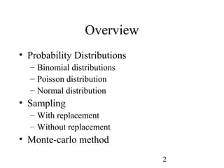
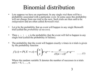
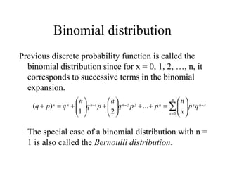
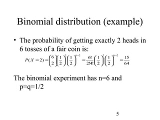
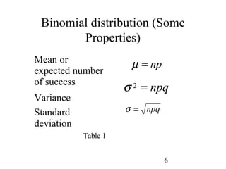
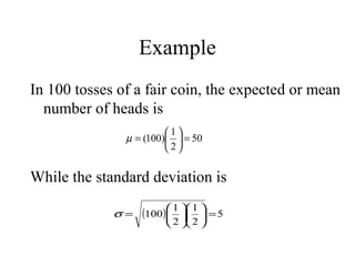
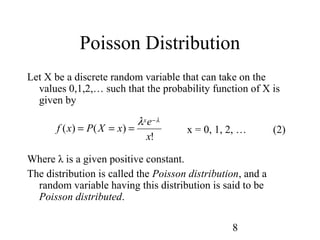
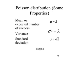
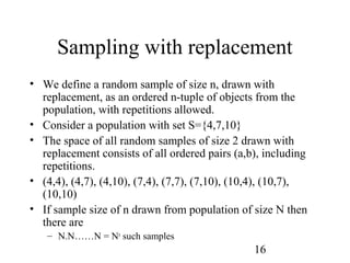
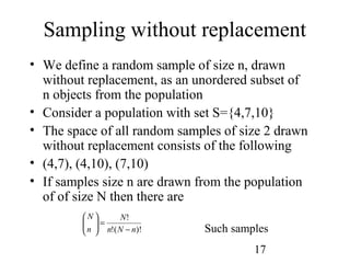
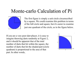
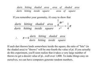
The document discusses various probability distributions including the binomial, Poisson, and normal distributions. It provides definitions and key properties of each distribution. It also discusses sampling with and without replacement as well as the Monte Carlo method for simulating physical systems using random sampling. The Monte Carlo method can be used to computationally estimate values like pi by simulating the throwing of darts at a circular target.

1. 1
Probability Distribution

2. 2
Overview
• Probability Distributions
– Binomial distributions
– Poisson distribution
– Normal distribution
• Sampling
– With replacement
– Without replacement
• Monte-carlo method

3. 3
Binomial distribution
• Lets suppose we have an experiment. In any single trial there will be a
probability associated with a particular event. In some cases this probability
will not change from one trial to the next. Such trials are then said to be
independent and are often called Bernoulli trial.
• Let p be the probability that an event will happen in any single Bernoulli
trial (called the probability of success).
• Then q = 1 - p is the probability that the event will fail to happen in any
single trial (called the probability of failure).
• The probability that the event will happen exactly x times in n trials is given
by the probability function
…….(1)
Where the random variable X denotes the number of successes in n trials
and x = 0, 1, …, n.
xnxxnx qp
xnx
n
qp
x
n
xXPxf −−
−
=





===
)!(!
!
)()(

4. Binomial distribution
Previous discrete probability function is called the
binomial distribution since for x = 0, 1, 2, …, n, it
corresponds to successive terms in the binomial
expansion.
The special case of a binomial distribution with n =
1 is also called the Bernoulli distribution.
∑=
−−−






=++





+





+=+
n
x
xnxnnnnn qp
x
n
ppq
n
pq
n
qpq
0
221 ...
21
)(

5. 5
Binomial distribution (example)
• The probability of getting exactly 2 heads in
6 tosses of a fair coin is:
The binomial experiment has n=6 and
p=q=1/2
64
15
2
1
2
1
!4!2
!6
2
1
2
1
2
6
)2(
262262
=











=

















==
−−
XP

6. 6
Binomial distribution (Some
Properties)
np=µ
npq=2σ
npq=σ
Mean or
expected number
of success
Variance
Standard
deviation
Table 1

7. Example
In 100 tosses of a fair coin, the expected or mean
number of heads is
While the standard deviation is
50
2
1
)100( =





=µ
( ) 5
2
1
2
1
100 =











=σ

8. 8
Poisson Distribution
Let X be a discrete random variable that can take on the
values 0,1,2,… such that the probability function of X is
given by
x = 0, 1, 2, … (2)
Where λ is a given positive constant.
The distribution is called the Poisson distribution, and a
random variable having this distribution is said to be
Poisson distributed.
!
)()(
x
e
xXPxf
x λλ −
===

9. 9
Poisson distribution (Some
Properties)
λµ =
λσ =2
λσ =
Mean or
expected number
of success
Variance
Standard
deviation
Table 2

10. 10
Relation Between Binomial and
Poisson Distribution
• In the binomial distribution (1), if n is large while the
probability p of occurrence of an event is close to zero, so
that q = 1 – p is close to 1, the event is called a rare
event.
• In practice we consider an event as rare if the number of
trials is at least 50 (n ≥ 50) while np is less than 5.
• For such cases the binomial distribution is very closely
approximated by the Poisson distribution (2) with λ = np, q
= 1, and p ≈ 1 in Table 1, we get the result in table 2.

11. 11
Normal Distribution
• One of the most important examples of a
continuous probability distribution is the
normal distribution, sometimes called the
Gaussian distribution. The density function
for this distribution is given by
………….(3)22 2/)(
2
1
)( σµ
πσ
−−= xexf

12. Normal Distribution (Some
Properties)
Mean expected value μ
Variance σ2
Standard deviation σ
Table 3

13. 13
Relation between Binomial and
Normal Distribution
• If n is large and if neither p nor q is too close to zero, the
binomial distribution can be closely approximated by a
normal distribution with standardized random variable
given by
Here X is the random variable giving the number of
successes in n Bernoulli trials and p is the probability of
success.
• The theoretical justification for the approximation of B(n,p)
by N(np, npq) is the fundamental central limit theorem
npq
npX
Z
−
=

14. 14
Sampling Distribution
(Population and Sample, Statistical Inference)
• Often in practice we are interested in drawing valid conclusions about
a large group of individuals or objects.
• Instead of examining the entire group, called the population, which
may be difficult or impossible to do, we may examine only a small
part of this population, which is called a sample.
• We do this with the aim of inferring certain facts about the population
from results found in the sample, a process known as statistical
inference.
• The process of obtaining samples is called sampling.
• Example: We may wish to draw conclusions about the heights (or
weights) of 12,000 adult students (the population) by examining only
100 students (a sample) selected from this population.

15. 15
Sampling Distribution
(Sampling with and without Replacement)
• If we draw object from an urn, we have the choice of replacing or
replacing the object into the urn before we draw again.
• When it is sure that each member of the population has the same
chance of being in the sample, which is then often called a random
sample.
• We consider two types of random samples
– Those drawn with replacement
– Those drawn without replacement
• The probability distribution of a random variable defined on a space of
random samples is called sampling distribution

16. 16
Sampling with replacement
• We define a random sample of size n, drawn with
replacement, as an ordered n-tuple of objects from the
population, with repetitions allowed.
• Consider a population with set S={4,7,10}
• The space of all random samples of size 2 drawn with
replacement consists of all ordered pairs (a,b), including
repetitions.
• (4,4), (4,7), (4,10), (7,4), (7,7), (7,10), (10,4), (10,7),
(10,10)
• If sample size of n drawn from population of size N then
there are
– N.N……N = Nn
such samples

17. 17
Sampling without replacement
• We define a random sample of size n, drawn
without replacement, as an unordered subset of
n objects from the population
• Consider a population with set S={4,7,10}
• The space of all random samples of size 2 drawn
without replacement consists of the following
• (4,7), (4,10), (7,10)
• If samples size n are drawn from the population
of of size N then there are
Such samples)!(!
!
nNn
N
n
N
−
=






18. 18
Monte-carlo method
• Monte carlo methods are class of computational algorithms
that rely on repeated random sampling
• These methods are often used when simulating physical
and mathematical systems
• There is not single Monte carlo method; instead the term
describes large and widely used class of approaches. These
approaches tend to follow a pattern
– Define a domain of possible inputs.
– Generate inputs randomly from the domain.
– Perform a deterministic computation using the inputs.
– Aggregate the results of the individual computations into the final
result

19. 19
Monte-carlo method
• Applications where these methods are used
– Physical science
– Design and visuals
– Finance and business
– Telecommunications
– Games
• Use in mathematics
– Integration
– Optimization etc.

20. Monte-carlo Calculation of Pi
The first figure is simply a unit circle circumscribed
by a square. We could examine this problem in terms
of the full circle and square, but it's easier to examine
just one quadrant of the circle, as in the figure below.
If you are a very poor dart player, it is easy to
imagine throwing darts randomly at Figure 2,
and it should be apparent that of the total
number of darts that hit within the square, the
number of darts that hit the shaded part (circle
quadrant) is proportional to the area of that
part. In other words,

21. squareofarea
areashadedofarea
squareinsidehittingdarts
areashadedhittingdarts
=
π
π
4
14
1
2
2
==
r
r
squareinsidehittingdarts
areashadedhittingdarts
If you remember your geometry, it's easy to show that
squareinsidehittingdarts
areashadedhittingdarts
4=∴ π
If each dart thrown lands somewhere inside the square, the ratio of "hits" (in
the shaded area) to "throws" will be one-fourth the value of pi. If you actually
do this experiment, you'll soon realize that it takes a very large number of
throws to get a decent value of pi...well over 1,000. To make things easy on
ourselves, we can have computers generate random numbers.

22. 22
References
• Introduction to probability and statistics
– Schaum’s series
• Proabability and statistics for engineers and
the sciences
– Jay L. Devore
• http://en.wikipedia.org/wiki