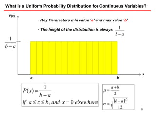
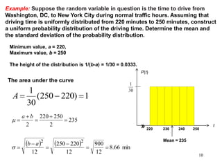
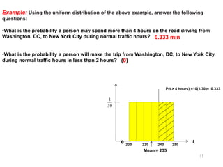
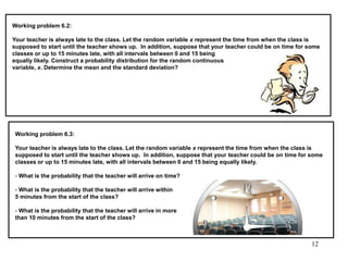
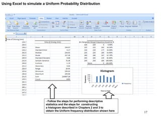
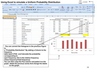
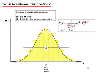
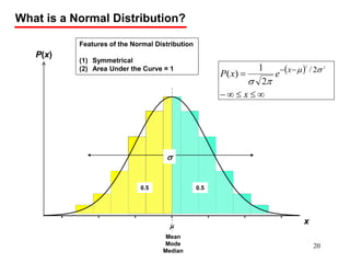
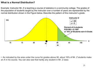
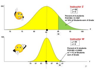
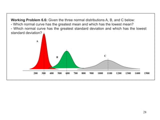
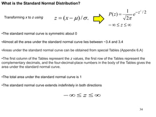
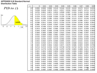
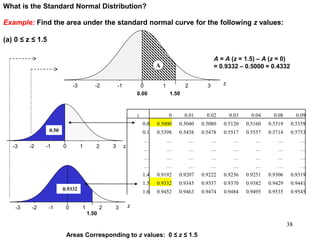
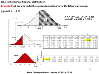
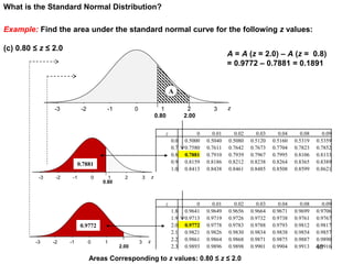
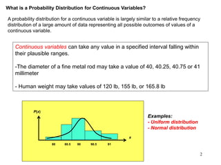
The document discusses probability distributions for continuous variables, explaining that continuous variables can take any value within a range and probability distributions depict the relative likelihood of these values being observed, with examples given of uniform and normal distributions and how they are characterized by parameters like mean and standard deviation. It also provides examples of how uniform and normal distributions can model real-world scenarios involving continuous variables like time or test scores.

1. PROBABILITY DISTRIBUTIONS
Part II: Probability Distributions for Continuous Variables
1

2. Continuous variables can take any value in a specified interval falling within
their plausible ranges.
-The diameter of a fine metal rod may take a value of 40, 40.25, 40.75 or 41
millimeter
- Human weight may take values of 120 lb, 155 lb, or 165.8 lb
What is a Probability Distribution for Continuous Variables?
A probability distribution for a continuous variable is largely similar to a relative frequency
distribution of a large amount of data representing all possible outcomes of values of a
continuous variable.
Examples:
- Uniform distribution
- Normal distribution
x
P(x)
80 80.5 90 90.5 91
2

3. What is a Probability Distribution for Continuous Variables?
Student
grades (%)
Mid-point
(x)
Number of
students
(frequency, f)
Relative
frequency
(RF)
20 to < 30 25 16 0.0032
30 to < 40 35 20 0.004
40 to < 50 45 98 0.0196
50 to < 60 55 256 0.0512
60 to < 70 65 1490 0.298
70 to < 80 75 1675 0.335
80 to < 90 85 1111 0.2222
90 to < 100 95 334 0.0668
N = 5000 Sum = 1
Example: Suppose 5000 students took
a course on statistics in a college over
the last 5 years. The categories of grades
and corresponding frequencies are as
shown in the Table below.
Construct a probability distribution of
Student’s grade.
0
0.05
0.1
0.15
0.2
0.25
0.3
0.35
0.4
20 to < 30 30 to < 40 40 to < 50 50 to < 60 60 to < 70 70 to < 80 80 to < 90 90 to < 100
P(x)
Grade Classes
A = 1
3

4. Example: Suppose 5000 students took a course on statistics in a college over
the last 5 years. The categories of grades and corresponding frequencies are as
shown in the Table below. Calculate the mean and variance of students’ grades.
Student
Grades (%)
Mid-
Point (x)
Number of
students-
(frequency, f)
Relative
Frequency
p(x) x.p(x) (x-m)2 p(x). (x-m)2
20 to < 30 25 16 0.0032 0.08 2366.43 7.57
30 to < 40 35 20 0.004 0.14 1493.51 5.97
40 to < 50 45 98 0.0196 0.88 820.59 16.08
50 to < 60 55 256 0.0512 2.82 347.67 17.8
60 to < 70 65 1490 0.298 19.37 74.75 22.28
70 to < 80 75 1675 0.335 25.13 1.83 0.61
80 to < 90 85 1111 0.2222 18.89 128.91 28.64
90 to < 100 95 334 0.0668 6.35 455.99 30.46
N = 5000 Sum = 1
Mean =
73.65
Variance
= 129.43
 )(xxPm
  222
)()](.)[( mm xPxxpx
Standard Deviation
= SQRT(129.43)
4

5. Working problem 6.1:
The table below represents different categories of property tax of a large population
of houses in New Jersey.
- Plot the probability distribution
- Calculate the expected value
- Calculate the variance
5

6. What is a Uniform Probability Distribution for Continuous Variables?
This is the simplest type of probability distribution for continuous variables and it can be used to
model both discrete and continuous variables. It is rectangular in shape as a result of the fact that
different data classes exhibit the same frequency or relative frequency.
P(x)
x
P(x)
x
Continuous Uniform Distribution Discrete Uniform Distribution
120 125 130 135 140
6

7. What is a Uniform Probability Distribution for Continuous Variables?
Examples: P(x)
x
•The time to fly via a commercial airliner from Newark airport to
Atlanta, Georgia, ranges from 120 minutes to 140 minutes.
If you monitor the fly time for many commercial flights it will
follow more or less a uniform distribution
•The time students take to finish one-hour standard test
may range from 50 minutes to 60 minutes. Equal numbers
of students complete the test over the 4 minutes intervals
within this range, 50, 54, 56, 58, and 60.
The finishing time of the test can be approximated
by a uniform distribution
• Time for pizza delivery by a certain restaurant
to a certain region in town may range from
20 minutes to 30 minutes from the time the
delivery man leaves the store.
7

8.  The time to fly via a commercial airliner from one airport to
another, say from Raleigh, North Carolina to Atlanta, Georgia.
This time may range from 55 minutes to 65 minutes. If you
monitor the fly time for many commercial flights it will follow
more or less a uniform distribution.
The time a student takes to finish one-hour standard test
may range from 50 minutes to 60 minutes. Approximately,
equal numbers of students complete the test over the 4 minutes
intervals within this range, 48, 52, 56, and 60. Thus, the
finishing time of the test can be approximated by a uniform
distribution
Examples of variables following a Uniform Distribution:
The time to deliver a pizza to a certain location in town may
range from 20 minutes to 30 minutes from the time the delivery
person leaves the store. This can be approximated by a
uniform distribution
The waiting time for a school bus may range from 20 minutes to 30
minutes. Within this period, waiting time can be approximated by a
uniform distribution.
8

9. a b
ab 
1
P(x)
x
What is a Uniform Probability Distribution for Continuous Variables?
elsewherexandbxaif
ab
xP
0,
1
)(



• Key Parameters min value ‘a’ and max value ‘b’
• The height of the distribution is always
ab 
1
 
12
2
2
ab
ba





m
9

10. Example: Suppose the random variable in question is the time to drive from
Washington, DC, to New York City during normal traffic hours. Assuming that
driving time is uniformly distributed from 220 minutes to 250 minutes, construct
a uniform probability distribution of the driving time. Determine the mean and
the standard deviation of the probability distribution.
Minimum value, a = 220,
Maximum value, b = 250
The height of the distribution is 1/(b-a) = 1/30 = 0.0333.
220 230 240 250
30
1
P(t)
t»
Mean = 235
1)220250(
30
1
A
The area under the curve
    min66.8
12
900
12
220250
12
235
2
250220
2
22










ab
ba

m
10

11. Example: Using the uniform distribution of the above example, answer the following
questions:
•What is the probability a person may spend more than 4 hours on the road driving from
Washington, DC, to New York City during normal traffic hours?
•What is the probability a person will make the trip from Washington, DC, to New York City
during normal traffic hours in less than 2 hours?
220 230 240 250
30
1
t»
Mean = 235
P(t > 4 hours) =10(1/30)= 0.333
0.333 min
(0)
11

12. Working problem 6.2:
Your teacher is always late to the class. Let the random variable x represent the time from when the class is
supposed to start until the teacher shows up. In addition, suppose that your teacher could be on time for some
classes or up to 15 minutes late, with all intervals between 0 and 15 being
equally likely. Construct a probability distribution for the random continuous
variable, x. Determine the mean and the standard deviation?
Working problem 6.3:
Your teacher is always late to the class. Let the random variable x represent the time from when the class is
supposed to start until the teacher shows up. In addition, suppose that your teacher could be on time for some
classes or up to 15 minutes late, with all intervals between 0 and 15 being equally likely.
- What is the probability that the teacher will arrive on time?
- What is the probability that the teacher will arrive within
5 minutes from the start of the class?
- What is the probability that the teacher will arrive in more
than 10 minutes from the start of the class?
12

13. Working problem 6.4:
Waiting period to see your eye doctor can be considered as a random
variable x representing the time from signing in to the time you actually
see the doctor. Further suppose that your doctor could see you as soon
as you sign in (x = 0) or up to 30 minutes late (x = 30) with all intervals
between 0 and 30 being equally likely. Construct a probability distribution
for the random continuous variable, x. Determine the mean and the
standard deviation?
Working problem 6.5:
Waiting period to see your eye doctor can be considered as a random variable x representing the time
from signing in to the time you actually see the doctor. Further suppose that your doctor could see you as
soon as you sign in (x = 0) or up to 30 minutes late (x = 30) with all intervals between 0 and 30 being
equally likely.
- What is the probability that your eye doctor will see you between 10 and 20 minutes?
- What is the probability that your eye doctor will see you in less than 5 minutes?
13

14. Using Excel to simulate a Uniform Probability Distribution
2
Go to Data
3
Go to Data Analysis
1
Type a label
Named “Time of
Driving”
4Go to Random Number Generation
5
Press OK
Example: Suppose the random variable in question is the time to drive from
Washington, DC, to New York City during normal traffic hours. Assuming that
driving time is uniformly distributed from 220 minutes to 250 minutes, construct
a uniform probability distribution of the driving time. Determine the mean and
the standard deviation of the probability distribution.
14

15. - Select 1 variable
- Select, say 1000 random numbers
- Select Uniform Distribution
- You will be prompted to insert
Uniform distribution parameters
(220 and 250 for this example)
- Specify an output right under the
label
6
7
Press OK
Using Excel to simulate a Uniform Probability Distribution
15

16. - The output of the analysis of
will be a long column of 1000 random
numbers representing random
values of driving time from
Washington, DC, to New York City
during normal traffic hours
Note: decimals are rounded off to one
Using Excel to simulate a Uniform Probability Distribution
16

17. - Follow the steps for performing descriptive
statistics and the steps for constructing
a histogram described in Chapters 2 and 3 to
obtain the Uniform frequency distribution shown here
Using Excel to simulate a Uniform Probability Distribution
17

18. - You can convert the histogram in the previous Figure
to
a “Probability Distribution” By adding a Column to the
frequency
table label it P(X) and Calculate the probability
corresponding to
each frequency, this is the relative frequency
(Class frequency/Total frequency)
You can then copy the P(x) column and paste it on the
graph, delete the previous series And change the labels
on the graph.
163.0
1000
163
Using Excel to simulate a Uniform Probability Distribution
18

19. What is a Normal Distribution?
 

 
x
exP x 22
2/
2
1
)( m

Features of the Normal Distribution
(1) Bell-Shaped
(2) Defined by two parameters, m and 
x
P(x)
Mean
Mode
Median

m
19

20. What is a Normal Distribution?
 

 
x
exP x 22
2/
2
1
)( m

Features of the Normal Distribution
(1) Symmetrical
(2) Area Under the Curve = 1
x
P(x)
Mean
Mode
Median

0.50.5
m
20

21. What is a Normal Distribution?
Examples of random variables following a normal distribution include:
 People’s income in a given nation- few earn low income, few earn high income,
and the majority earns middle income.
 Students’ grades in a course- few earn low grades, few earn high grades, and
the majority earns middle grades.
 People’s height- few are short, few are tall, and the majority has middle
heights.
 Education cost- some colleges charge small tuition, some charge very high
tuition, and the majority charges tuition in between.
21

22. Example: Given the three normal distributions a, b, and C below:
- Which normal curve has the greatest mean and which has the lowest mean?
- Which normal curve has the greatest standard deviation and which has the lowest standard
deviation?
-20 0 20 40 60 80 100 120 140 160 180 200 220
A
B
C
Solution:
Distribution A: Mean ≈ 30
Distribution B: Mean ≈ 80
Distribution C: Mean ≈ 160
Distribution C is the most spread out distribution. Therefore, it has the greatest standard deviation.
Distribution B is the least spread out distribution. Therefore, it has the lowest standard deviation.
22

23. Recall: The Empirical Rule
What is a Normal Distribution?
RelativeFrequency(%)
Mean
Mode
Median
m +/- 3 
m +/- 2 
99.74%
95.44%
m +/- 1 
68.26%
x
23

24. What is a Normal Distribution?
Example: Instructor Mr. Z is teaching a course of statistics in a community college. The grades of
the population of students taught by the instructor over a number of years are represented by the
normal distribution shown in the Figure below. Describe the pattern of this instructor’s grade.
100959085807570
f(X)
X
• As can be seen in this Figure, the grades given by Mr. Z follows a normal distribution
with mean of 85 and a standard deviation of 5. This means that Mr. Z’s average grade
is a B and also most of his students earn a B grade (the mode).
Using the empirical rule:
•About 68.26 % of Mr. Z’s class earn grades from 80 to 90 (m ± 1)
•About 95.44% of Mr. Z’s class earn grades from 75 to 95 (m ± 2)
•About 99.74% of Mr. Z’s class earn grades from 70 to 100 (m ± 3)
•Virtually, no student fails Mr. Z’s class as the percent of students earning less than 50% is zero.24

25. What is a Normal Distribution?
Example: Instructor Mr. Z is teaching a course of statistics in a community college. The grades of
the population of students taught by the instructor over a number of years are represented by the
normal distribution shown in the Figure below. Describe the pattern of this instructor’s grade.
100959085807570
f(X)
X
90
• As indicated by the area under the curve for grades above 90, about 16% of Mr. Z students make
an A in his course. You can also see that hardly any student in Mr. Z class
Instructor Z
m = 85
 = 5
Percent of A students
P(G>90) = 0.1587
or 16% of Students earn A Grade
25

26. Example: Suppose we want to compare the grades of Mr. Z with those of another instructor, Mr. W
who is teaching the same course for different groups of students. The grades of the populations of
students taught by the two instructors are represented by the two normal distributions shown in the
next slide. Note that we are also looking at the percent of students making A grade taught by each
instructor. Describe the two normal distributions and compare the grades by the two instructors. If
you have a choice to take the statistics course by either instructor, which one would you chose to
take the course with?
What is a Normal Distribution?
26

27. 100959085807570
f(X)
X
90
Instructor Z
m = 85
 = 5
Percent of A students
P(G>90) = 0.1587
or 16% of Students earn A Grade
f(X)
X
91898785838179
90
Instructor W
m = 85
 = 2
Percent of A students
P(G>90) = 0.0062
or < 1% of Students
earn A Grade
27

28. 200 300 400 500 600 700 800 900 1000 1100 1200 1300 1400 1500
A
C
B
Working Problem 6.6: Given the three normal distributions A, B, and C below:
- Which normal curve has the greatest mean and which has the lowest mean?
- Which normal curve has the greatest standard deviation and which has the lowest
standard deviation?
28

29. Working Problem 6.7: The two normal distributions below describe the area (cm2) of ceramic tiles produced by two
manufacturers A & B:
- Compare the mean and the variability of the two distributions
- Which manufacturer should you buy ceramic tiles from?
16.616.416.216.015.815.615.4
Area (cm2)
m = 16
 = 0.2
Manufacturer A
18.417.616.816.015.214.413.6
m = 16
 = 0.8
Area (cm2)
Manufacturer B
29

30. Review Problem 6.1:
The frequency distribution given below represents the heights of 1000 students in a college.
- Perform descriptive statistics to Prove whether this distribution can be approximated by a normal distribution.
- Determine, the mean, the median, the mode, and the standard deviation
- Given that this distribution is indeed normal, use the empirical rule to determine the
heights of 68.26% of the students , the heights of 95.44% of the students , and the heights of 99.74% of the students ,
lower
Heights (cm)
upper midpoint frequency
130 < 135 133 0
135 < 140 138 4
140 < 145 143 15
145 < 150 148 37
150 < 155 153 64
155 < 160 158 125
160 < 165 163 190
165 < 170 168 196
170 < 175 173 161
175 < 180 178 97
180 < 185 183 75
185 < 190 188 28
190 < 195 193 7
195 < 200 197 1
1000
30

31. What is the Standard Normal Distribution?
3210-1-2-3
f(z)
z
Mean = m = 0
68.26%
95.44%
99.74%
Transforming x to z using ./)( m xz

 
z
ezP z 2/2
2
1
)(

Standard Deviation
 = 1
A normal distribution having mean 0 and standard deviation 1 is said to be a
standard normal distribution.
31

32. The basic properties of the standard normal distribution:
•The total area under the standard normal curve is one.
•The standard normal curve extends indefinitely in both directions ( )
•The standard normal curve is symmetric about 0.
•Almost all the area under the standard normal curve lies between values of z of −3.4 and 3.4.
•Areas under the standard normal curve can be obtained from special tables such as the ones
shown in Appendix 6.A.
32

33. 3210-1-2-3
f(z)
z
-1.50
A= 0.0668
3210-1-2-3
f(z)
z
1.50
A= 0.9332
z 0 0.01 0.02 0.03 0.04 0.05 0.06 0.07 0.08 0.09
-3.4 0.0003 0.0003 0.0003 0.0003 0.0003 0.0003 0.0003 0.0003 0.0003 0.0002
-3.3 0.0005 0.0005 0.0005 0.0004 0.0004 0.0004 0.0004 0.0004 0.0004 0.0003
-3.2 0.0007 0.0007 0.0006 0.0006 0.0006 0.0006 0.0006 0.0005 0.0005 0.0005
.. .. .. .. .. .. .. .. .. .. ..
-1.5 0.0668 0.0655 0.0643 0.0630 0.0618 0.0606 0.0594 0.0582 0.0571 0.0559
-1.4 0.0808 0.0793 0.0778 0.0764 0.0749 0.0735 0.0721 0.0708 0.0694 0.0681
.. .. .. .. .. .. .. .. .. .. ..
0.0 0.5000 0.4960 0.4920 0.4880 0.4840 0.4801 0.4761 0.4721 0.4681 0.4641
z 0 0.01 0.02 0.03 0.04 0.05 0.06 0.07 0.08 0.09
0.0 0.5000 0.5040 0.5080 0.5120 0.5160 0.5199 0.5239 0.5279 0.5319 0.5359
.. .. .. .. .. .. .. .. .. .. ..
1.4 0.9192 0.9207 0.9222 0.9236 0.9251 0.9265 0.9279 0.9292 0.9306 0.9319
1.5 0.9332 0.9345 0.9357 0.9370 0.9382 0.9394 0.9406 0.9418 0.9429 0.9441
1.6 0.9452 0.9463 0.9474 0.9484 0.9495 0.9505 0.9515 0.9525 0.9535 0.9545
.. .. .. .. .. .. .. .. .. .. ..
3.2 0.9993 0.9993 0.9994 0.9994 0.9994 0.9994 0.9994 0.9995 0.9995 0.9995
Construction of the Standard Normal Table
Area Values
33

34. What is the Standard Normal Distribution?

 
z
ezP z 2/2
2
1
)(
Transforming x to z using ./)( m xz
•The total area under the standard normal curve is 1
•The standard normal curve extends indefinitely in both directions
 z
•The standard normal curve is symmetric about 0
•Almost all the area under the standard normal curve lies between −3.4 and 3.4
•Areas under the standard normal curve can be obtained from special Tables (Appendix 6.A)
•The first column of the Tables represent the z values, the first row of the Tables represent the
complementary decimals, and the four-decimal-place numbers in the body of the Tables gives the
area under the standard normal curve.
34

35. ®Quality Business Consulting-QBC, 2010
35

36. QBC
®
®Quality Business Consulting-QBC, 2010
36

37. z 0 0.01 0.02 0.03 0.04 0.05 0.06 0.07 0.08 0.09
0.0 0.0000 0.0040 0.0080 0.0120 0.0160 0.0199 0.0239 0.0279 0.0319 0.0359
0.1 0.0398 0.0438 0.0478 0.0517 0.0557 0.0596 0.0636 0.0675 0.0714 0.0753
0.2 0.0793 0.0832 0.0871 0.0910 0.0948 0.0987 0.1026 0.1064 0.1103 0.1141
0.3 0.1179 0.1217 0.1255 0.1293 0.1331 0.1368 0.1406 0.1443 0.1480 0.1517
0.4 0.1554 0.1591 0.1628 0.1664 0.1700 0.1736 0.1772 0.1808 0.1844 0.1879
0.5 0.1915 0.1950 0.1985 0.2019 0.2054 0.2088 0.2123 0.2157 0.2190 0.2224
0.6 0.2257 0.2291 0.2324 0.2357 0.2389 0.2422 0.2454 0.2486 0.2517 0.2549
0.7 0.2580 0.2611 0.2642 0.2673 0.2704 0.2734 0.2764 0.2794 0.2823 0.2852
0.8 0.2881 0.2910 0.2939 0.2967 0.2995 0.3023 0.3051 0.3078 0.3106 0.3133
0.9 0.3159 0.3186 0.3212 0.3238 0.3264 0.3289 0.3315 0.3340 0.3365 0.3389
1.0 0.3413 0.3438 0.3461 0.3485 0.3508 0.3531 0.3554 0.3577 0.3599 0.3621
1.1 0.3643 0.3665 0.3686 0.3708 0.3729 0.3749 0.3770 0.3790 0.3810 0.3830
1.2 0.3849 0.3869 0.3888 0.3907 0.3925 0.3944 0.3962 0.3980 0.3997 0.4015
1.3 0.4032 0.4049 0.4066 0.4082 0.4099 0.4115 0.4131 0.4147 0.4162 0.4177
1.4 0.4192 0.4207 0.4222 0.4236 0.4251 0.4265 0.4279 0.4292 0.4306 0.4319
1.5 0.4332 0.4345 0.4357 0.4370 0.4382 0.4394 0.4406 0.4418 0.4429 0.4441
1.6 0.4452 0.4463 0.4474 0.4484 0.4495 0.4505 0.4515 0.4525 0.4535 0.4545
1.7 0.4554 0.4564 0.4573 0.4582 0.4591 0.4599 0.4608 0.4616 0.4625 0.4633
1.8 0.4641 0.4649 0.4656 0.4664 0.4671 0.4678 0.4686 0.4693 0.4699 0.4706
1.9 0.4713 0.4719 0.4726 0.4732 0.4738 0.4744 0.4750 0.4756 0.4761 0.4767
2.0 0.4772 0.4778 0.4783 0.4788 0.4793 0.4798 0.4803 0.4808 0.4812 0.4817
2.1 0.4821 0.4826 0.4830 0.4834 0.4838 0.4842 0.4846 0.4850 0.4854 0.4857
2.2 0.4861 0.4864 0.4868 0.4871 0.4875 0.4878 0.4881 0.4884 0.4887 0.4890
2.3 0.4893 0.4896 0.4898 0.4901 0.4904 0.4906 0.4909 0.4911 0.4913 0.4916
2.4 0.4918 0.4920 0.4922 0.4925 0.4927 0.4929 0.4931 0.4932 0.4934 0.4936
2.5 0.4938 0.4940 0.4941 0.4943 0.4945 0.4946 0.4948 0.4949 0.4951 0.4952
2.6 0.4953 0.4955 0.4956 0.4957 0.4959 0.4960 0.4961 0.4962 0.4963 0.4964
2.7 0.4965 0.4966 0.4967 0.4968 0.4969 0.4970 0.4971 0.4972 0.4973 0.4974
2.8 0.4974 0.4975 0.4976 0.4977 0.4977 0.4978 0.4979 0.4979 0.4980 0.4981
2.9 0.4981 0.4982 0.4982 0.4983 0.4984 0.4984 0.4985 0.4985 0.4986 0.4986
3.0 0.4987 0.4987 0.4987 0.4988 0.4988 0.4989 0.4989 0.4989 0.4990 0.4990
310-1-2-3
f(z)
z
1.96
0.4750
APPENDIX 6.B Standard Normal
Distribution Table
)0( ztoP
37

38. Example: Find the area under the standard normal curve for the following z values:
(a) 0 ≤ z ≤ 1.5
What is the Standard Normal Distribution?
3210-1-2-3 z
1.500.00
A = A (z = 1.5) – A (z = 0)
= 0.9332 – 0.5000 = 0.4332A
Areas Corresponding to z values: 0 ≤ z ≤ 1.5
z 0 0.01 0.02 0.03 0.04 0.08 0.09
0.0 0.5000 0.5040 0.5080 0.5120 0.5160 0.5319 0.5359
0.1 0.5398 0.5438 0.5478 0.5517 0.5557 0.5714 0.5753
… … … … … … … …
… … … … … … … …
… … … … … … … …
… … … … … … … …
1.4 0.9192 0.9207 0.9222 0.9236 0.9251 0.9306 0.9319
1.5 0.9332 0.9345 0.9357 0.9370 0.9382 0.9429 0.9441
1.6 0.9452 0.9463 0.9474 0.9484 0.9495 0.9535 0.9545
3210-1-2-3 z
1.50
0.9332
3210-1-2-3 z
0.50
38

39. Example: Find the area under the standard normal curve for the following z values:
(b) –0.46 ≤ z ≤ 2.30
What is the Standard Normal Distribution?
3210-1-2-3 z
2.30-0.46
A = A (z = 2.3) – A (z = -0.46)
= 0.9893 – 0.3228 = 0.6665A
Areas Corresponding to z values: –0.46 ≤ z ≤ 2.30
z 0 0.01 0.02 0.03 0.04 0.05 0.06 0.07 0.09
2.3 0.9893 0.9896 0.9898 0.9901 0.9904 0.9906 0.9909 0.9911 0.9916
2.4 0.9918 0.9920 0.9922 0.9925 0.9927 0.9929 0.9931 0.9932 0.9936
z 0 0.01 0.02 0.03 0.04 0.05 0.06 0.09
-0.5 0.3085 0.305 0.3015 0.2981 0.2946 0.2912 0.2877 0.2776
-0.4 0.3446 0.3409 0.3372 0.3336 0.33 0.3264 0.3228 0.3121
-0.3 0.3821 0.3783 0.3745 0.3707 0.3669 0.3632 0.3594 0.3483
-0.2 0.4207 0.4168 0.4129 0.409 0.4052 0.4013 0.3974 0.3859
-0.1 0.4602 0.4562 0.4522 0.4483 0.4443 0.4404 0.4364 0.4247
0 0.5 0.496 0.492 0.488 0.484 0.4801 0.4761 0.4641
3210-1-2-3 z
2.30
0.9893
3210-1-2-3 z-0.46
0.3228
39

40. Example: Find the area under the standard normal curve for the following z values:
(c) 0.80 ≤ z ≤ 2.0
What is the Standard Normal Distribution?
A = A (z = 2.0) – A (z = 0.8)
= 0.9772 – 0.7881 = 0.1891
3210-1-2-3 z
2.000.80
A
Areas Corresponding to z values: 0.80 ≤ z ≤ 2.0
z 0 0.01 0.02 0.03 0.04 0.08 0.09
0.0 0.5000 0.5040 0.5080 0.5120 0.5160 0.5319 0.5359
0.7 0.7580 0.7611 0.7642 0.7673 0.7704 0.7823 0.7852
0.8 0.7881 0.7910 0.7939 0.7967 0.7995 0.8106 0.8133
0.9 0.8159 0.8186 0.8212 0.8238 0.8264 0.8365 0.8389
1.0 0.8413 0.8438 0.8461 0.8485 0.8508 0.8599 0.8621
z 0 0.01 0.02 0.03 0.04 0.08 0.09
1.8 0.9641 0.9649 0.9656 0.9664 0.9671 0.9699 0.9706
1.9 0.9713 0.9719 0.9726 0.9732 0.9738 0.9761 0.9767
2.0 0.9772 0.9778 0.9783 0.9788 0.9793 0.9812 0.9817
2.1 0.9821 0.9826 0.9830 0.9834 0.9838 0.9854 0.9857
2.2 0.9861 0.9864 0.9868 0.9871 0.9875 0.9887 0.9890
2.3 0.9893 0.9896 0.9898 0.9901 0.9904 0.9913 0.9916
310-1-2-3 z
2.00
0.9772
3210-1-2-3 z
0.80
0.7881
40

41. Example: Determine the value(s) of z in the following cases:
(a) Area under the normal curve between 0 and z is 0.3790.
What is the Standard Normal Distribution?
3210-1-2-3
z
1.170.00
0.5000
z 0 0.01 0.02 0.03 0.04 0.05 0.06 0.07 0.08 0.09
1.0 0.8413 0.8438 0.8461 0.8485 0.8508 0.8531 0.8554 0.8577 0.8599 0.8621
1.1 0.8643 0.8665 0.8686 0.8708 0.8729 0.8749 0.8770 0.8790 0.8810 0.8830
1.2 0.8849 0.8869 0.8888 0.8907 0.8925 0.8944 0.8962 0.8980 0.8997 0.9015
1.3 0.9032 0.9049 0.9066 0.9082 0.9099 0.9115 0.9131 0.9147 0.9162 0.9177
1.4 0.9192 0.9207 0.9222 0.9236 0.9251 0.9265 0.9279 0.9292 0.9306 0.9319
1.5 0.9332 0.9345 0.9357 0.9370 0.9382 0.9394 0.9406 0.9418 0.9429 0.9441
A= 0.879
0.3790
41

42. Example: Determine the value(s) of z in the following cases:
(b) Area under the normal curve to left of z is 0.6100.
What is the Standard Normal Distribution?
3210-1-2-3
f(z)
z
0.28
0.6100
z 0 0.01 0.02 0.03 0.04 0.05 0.06 0.07 0.08 0.09
0.0 0.5000 0.5040 0.5080 0.5120 0.5160 0.5199 0.5239 0.5279 0.5319 0.5359
0.1 0.5398 0.5438 0.5478 0.5517 0.5557 0.5596 0.5636 0.5675 0.5714 0.5753
0.2 0.5793 0.5832 0.5871 0.5910 0.5948 0.5987 0.6026 0.6064 0.6103 0.6141
0.3 0.6179 0.6217 0.6255 0.6293 0.6331 0.6368 0.6406 0.6443 0.6480 0.6517
0.4 0.6554 0.6591 0.6628 0.6664 0.6700 0.6736 0.6772 0.6808 0.6844 0.6879
0.5 0.6915 0.6950 0.6985 0.7019 0.7054 0.7088 0.7123 0.7157 0.7190 0.7224
0.6 0.7257 0.7291 0.7324 0.7357 0.7389 0.7422 0.7454 0.7486 0.7517 0.7549
0.7 0.7580 0.7611 0.7642 0.7673 0.7704 0.7734 0.7764 0.7794 0.7823 0.7852 42

43. Example: The mean value of course grades in a large population of students is 85, and the
standard deviation is 5, assuming that the grade follows a normal distribution, determine the z
values corresponding to the following grades:
• Grade = x = 75
• 80 ≤ x ≤ 90
• 75 ≤ x ≤ 95
• 70 ≤ x ≤ 100
Solution:
• At x = 75, z = (x-m)/ = (75-85)/5 = -2
• 80 ≤ x ≤ 90 yields (80-85)/5 ≤ z ≤ (90-85)/5, or -1 ≤ z ≤ +1
•75 ≤ x ≤ 95 yields (75-85)/5 ≤ z ≤ (95-85)/5, or -2 ≤ z ≤ +2
•70 ≤ x ≤ 100 yields (70-85)/5 ≤ z ≤ (100-85)/5, or -3 ≤ z ≤ +3
43

44. Example: In previous example. what percent of students made the following grades?
• 80 ≤ x ≤ 90
• 75 ≤ x ≤ 95
•70 ≤ x ≤ 100
Solution:
Using the empirical rule,
• 80 ≤ x ≤ 90 yields (80-85)/5 ≤ z ≤ (90-85)/5, or -1 ≤ z ≤ +1 and this corresponds to 68.26% of the
students’ grades.
• 75 ≤ x ≤ 95 yields (75-85)/5 ≤ z ≤ (95-85)/5, or -2 ≤ z ≤ +2 and this corresponds to 95.44% of the
students’ grades.
• 70 ≤ x ≤ 100 yields (70-85)/5 ≤ z ≤ (100-85)/5, or -3 ≤ z ≤ +3 and this corresponds to 99.74% of
the students’ grades.
44

45. -1 0 1 2 3 4 5 6 7 8 9 10 11 12 13 14 15 16 17 18 x
(A)
Mean = m = 2
Std. Dev. =  = 1
(B)
Mean = m = 6
Std. Dev. =  = 1/2
(C) Mean = m = 12
Std. Dev. =  = 2
Working Problem 6.8: For the three normal distributions shown below, find the values of z corresponding to the values of x in the circles
(A)
z= ?
(B)
z= ?
(C)
z= ?
45

46. Working Problem 6.9:
Find the area under the standard normal curve for the following z values:
(a) 0 ≤ z ≤ 1.0
(b) -2 ≤ z ≤ 2
(c) z < 3
Working Problem 6.10:
Find the area under the standard normal curve for the following z values:
(a) -∞ ≤ z ≤ 1.3
(b) -1 ≤ z ≤ 1.3
(c) z > -3.2
Working Problem 6.11:
Determine the value(s) of z in the following cases:
(a)Area under the normal curve between - ∞ and z is 0.100.
(b) Area under the normal curve to right of z is 0.8100.
(c) Area under the normal curve to left of z is 0.7100
46

47. Working Problem 6.12:
The three normal distributions shown below represent the grades of pre-algebra course of students obtained
in three different semesters…
- Describe and compare the performances of students in the three semester
- What percent of students failed (<60%) in each semester
m  75 m  80 m  85
  5   5   5
Working Problem 6.13:
The three normal distributions shown below represent the grades of pre-algebra course of students obtained
in three different semesters…
- Describe and compare the performances of students in the three semester
- What percent of students made at least B (≥ 80%) in each semester
m  75 m  80 m  85
  8   6   3
47

48. The za Notation
Example: Find the za values for the following cases:
• a = 0.01
• a = 0. 05
• a = 0.10
(a) a = 0.01 or 1%
1 – a = 0.99 or 99%
(a) za = z0.01 = 2.33
One-Sided
(b) a = 0.05 or 5%
1 – a = 0.95 or 95%
za = z0.05 = 1.64
One-Sided
(c) a = 0.10 or 10%
1 – a = 0.9 or 90%
za = z0.1 = 1.28
One-Sided
3210-1-2-3
z
A = 1- a = 0.90
or 90%
a = 0.10
za = 1.28
3210-1-2-3
z
a = 0.05
za = 1.64
A = 1- a = 0.95
or 95%
3210-1-2-3
z
za =2.33
a = 0.01A = 1- a = 0.99
or 99%
48

49. Example: Find the za/2 values for the following cases:
• a/2 = 0.005
• a/2 = 0. 025
• a/2 = 0.05
(a) a = 0.01 or 1%
1 – 2 a/2 = 0.99 or 99%
za/2 = z0.01/2 =
z0.005 = +/- 2.58
Two-Sided
(b) a = 0.05 or 5%
1 – 2 a/2 = 0.95 or 95%
za/2 = z0.05/2 =
z0.025 = +/- 1.96
Two-Sided
(c) a = 0.10 or 10%
1 – 2 a/2 = 0.90 or 90%
za/2 = z0.1/2 =
z0.05 = +/- 1.64
Two-Sided
3210-1-2-3 z
A = 1- a = 0.99
or 99%
za/2 = +2.58za/2 = -2.58
a/2 = 0.005
a/2 = 0.005
3210-1-2-3
z
A = 1- a = 0.95
or 95%
za/2 = +1.96za/2 = -1.96
a/2 = 0.025a/2 = 0.025
3210-1-2-3 z
A = 1- a = 0.90
or 90%
za/2 = +1.64za/2 = -1.64
a/2 = 0.05a/2 = 0.05
49

50. Applications of the standard normal distribution
In most applications dealing with the standard normal distribution require
the following basic steps:
Step 1: Sketch the normal curve associated with the variable to describe the problem in
question
Step 2: Shade the region of interest and mark its delimiting x-value(s).
Step 3: Calculate the z-score(s) corresponding to the x values:
.
:
.
Step 4: Use the standard normal distribution table to find the area under the standard
normal curve delimited by the z-score(s).
Step 5: Express the findings in terms of x values.
50

51. Example:
The Thermosense Company produces digital thermometers that have a
0oC midpoint, which is the reading expected at the freezing point of
water. In actual testing of a large number of thermometers, the temperature
at freezing points fluctuates around the 0oC from negative values (below 0oC)
to positive values (above 0oC). The temperature follows a normal distribution
with a mean value of 0oC and a standard deviation of 1oC. If one thermometer
is randomly selected, find the probability that, at the freezing point of water,
the reading is more than -1.2oC. What is the probability that, at the freezing
point of water, the reading is less than 0.5oC.
Solution:
With a mean value m = 0 and a standard deviation  = 1, this is a standard normal distribution.
Using the normal table in Appendix 6-A, we can find the area P(-∞ ≤ z ≤ -1.2), which is 0.1151 as
shown below. This yields value of P(z > -1.2) of 0.8849 (or 1- 0.1151). This answer means that the
chance that the reading at the freezing point of water will be more than -1.2oC is 0.8849 or about
88.5%.
z 0 0.01 0.02 0.03 0.04 0.05
-3.3 0.0005 0.0005 0.0005 0.0004 0.0004 0.0004
-1.4 … … … … … …
-1.3 0.0968 0.0951 0.0934 0.0918 0.0901 0.0885
-1.2 0.1151 0.1131 0.1112 0.1093 0.1075 0.1056
-1.1 0.1357 0.1335 0.1314 0.1292 0.1271 0.1251
-1.0 … … … … … …
3210-1-2-3 z
-1.20
0.8849
0.1151
51

52. What is the probability that, at the freezing point of water, the reading is
less than 0.5oC.
Solution:
The probability that, at the freezing point of water, the reading is less than 0.5oC
can be obtained using the normal table in Appendix 6-A, we can find the area
P(z < 0.5), which is 0.6915 as shown below. This answer means that the chance
that the reading at the freezing point of water will be less than 0.5oC is 0.6915
or about 69.15%.
z 0 0.01 0.02 0.03
0.0 0.5000 0.5040 0.5080 0.5120
… … … … …
0.5 0.6915 0.6950 0.6985 0.7019
0.6 0.7257 0.7291 0.7324 0.7357
3210-1-2-3 z
0.50
0.6915
0.3085
52

53. Working Problem 6.14: The property tax of houses in a large City in the State of New Jersey is
normally distributed. The normal curve shown below represents this distribution. What is the
mean value of property tax? Estimate the standard deviation of this normal distribution.
6,0005,5005,0004,5004,0003,5003,000
f(X)
x
53

54. Example: A sewing mill pays workers by the quantity of garments they make. The average annual
pay per worker is $18,000 and the standard deviation is $4000. Find the probability that a worker
selected randomly earns between $13,000 and $20,000.
Solution:
Following the procedure in the above example, the probability that a worker selected randomly
earns between $13,000 and $20,000 is calculated using the steps shown in Figure 6.20. As can
be seen in this Figure, this probability is 0.5859. This result also implies that about 58.6% of the
workers earn wages between $13,000 and $20,000.
30,00026,00022,00018,00014,00010,0006,000
f(x)
x
m = $18,000
 = $4000
3210-1-2-3
0.50-1.25
30,00026,00022,00018,00014,00010,0006,000
f(x)
x
20,00013,000
A=
?
0.5859
Finding the probability a worker selected earns between $13,000 and $20,000
54

55. Working Problem 6.15:
The weekly gross income of restaurant assistant managers follows a normal
distribution with a mean of $1,000 and a standard deviation of $100. The variation in
the weekly income of assistant managers is a result of managers getting a commission
in addition to their weekly salary.
- What are the z values for the income of assistant managers earning between $900 and
$1,100 weekly? What is the percent of assistant managers earning this range of income?
- What are the z values for the income of assistant managers earning between $800 and
$1,200 weekly? What is the percent of assistant managers earning this range of income?
- What are the z values for the income of assistant managers earning between $700 and
$1,100 weekly? What is the percent of assistant managers earning this range of income?
- What is the z value for the income of assistant managers earning less than $860 weekly?
What is the percent of assistant managers earning this range of income?
- What is the z value for the income of assistant managers earning more than $1,050 weekly?
What is the percent of assistant managers earning this range of income?
55

56. Example: According to the controversial 2002 book titled “IQ and the Wealth of Nations” by
Richard Lynn, and Tatu Vanhanen (Praeger/Greenwood Publication, Westport, Connecticut,
London, 2002),
The average IQ (Intelligence Quotient) test score of the world was 88 and the standard deviation
was 12. Using the following criteria typically describes one’s intelligence with respect to IQ score:
Applications of the Standard Normal Distribution
IQ Description
130+ Very superior
120-129 Superior
110-119 High average
90-109 Average
80-89 Low average
70-79 Borderline
Below 70 Extremely low
IQ Criteria
(http://iq-test.learninginfo.org/iq04.htm)
• Determine the percent of people in
the world that their intelligences are
considered above average or better
(IQ ≥ 110)?
• Determine the percent of people in
the world that their intelligences are
considered average (IQ = 90-109)?
56

57. Example:
m = 88
 = 12
Applications of the Standard Normal Distribution
IQ Description
130+ Very superior
120-129 Superior
110-119 High average
90-109 Average
80-89 Low average
70-79 Borderline
Below 70 Extremely low
IQ Criteria
(http://iq-test.learninginfo.org/iq04.htm)
• Determine the percent of people
in the world that their intelligences
are considered above
average or better (IQ ≥ 110)?
124112100766452
f( IQ)
IQ
m = 88
 = 12
(a)
12411210088766452
f(IQ)
IQ
110
(b)
3210-1-2-3
f(z)
z
z = 1.83
Area of interest
= 0.0336(c)
0.9664
1.83
57

58. Example:
m = 88
 = 12
Applications of the Standard Normal Distribution
IQ Description
130+ Very superior
120-129 Superior
110-119 High average
90-109 Average
80-89 Low average
70-79 Borderline
Below 70 Extremely low
IQ Criteria
(http://iq-test.learninginfo.org/iq04.htm)
• Determine the percent of people in
the world that their intelligences
are considered average
(IQ = 90-109)?
124112100766452
f( IQ)
IQ
m = 88
(a)
 = 12
10990
12411210088766452
f(IQ)
IQ
A=?
(b)
3210-1-2-3
f(z)
z
1.750.17
Area of interest
= 0.3920
(c)
58

59. Using Microsoft Excel® to find the Area under the Normal Distribution Curve
1
2
3
• Go to Excel Spreadsheet
• Click fx on the button bar
• Select Statistical from the “Or select a
category” drop down list box
•Select NORMDIST from the “Select a
function” list
• Click OK
Example:
Determine the area
to the left
(cumulative area) of
a certain value of x,
say 109 in a normal
distribution with mean
value of 88 and standard
deviation of 12.
59

60. 12411210088766452
f(X)
X
109
0.95994
4
•Type 109 in the X text box
•Click in the Mean text box and type 88
•Click in the Standard deviation text box and
type 12
•Click in the Cumulative text box and type TRUE
•You should be able to see the value of the area
as illustrated by the circle shown here, or you
can Click Ok and the value will be presented
60

61. Using Microsoft Excel® to Generate Random Numbers following a Normal Distribution
2
3
m

Example:
Sales Revenues
m = 100,000
 = 15000
Example: In the analysis of the net income of a textile company, it was found that the total sales revenues per
week of the company follows a normal distribution with a mean value of $100,000, and a standard deviation of
$15,000. Generate a normal distribution for the sales revenues per week using Microsoft Excel® data analysis.
61

62. Generated
Random
Values of
Sales Revenues
per month
5
4
62

63. 6
7
63

64. 64

65. 65