The document covers statistical inference, focusing on probability concepts, types of variables, and various important distributions such as Bernoulli, binomial, normal, and Poisson. It explains essential probability rules, joint and conditional probabilities, and Bayes' theorem, alongside methods for calculating expected values and variances. Additionally, it provides examples and applications of these concepts in real-world contexts, such as cancer detection and ad campaign performance.

1. Statistical Inference
Weeks 1 & 2: Probability and Distribution

2. Types of Variables
All Variables
Categorical
 May be represented by
numbers, but does not
make sense to add,
subtract, average, etc
Numerical
 Makes sense to add,
subtract, average, etc
(i.e., perform math
operations)
Discrete
 Are counted and can
only take on non-
negative whole numbers
Continuous
 Are measured and
can take on any real
number (i.e., have
decimal places)
Categorical
 Have no inherent
ordering (e.g.,
single, married,
divorced)
Ordinal
 Have ordered levels
(e.g., primary,
secondary, JC,
university, etc)

3. Probability
 P(A) = Probability of event A happening
0 ≤ P(A) ≤ 1
Disjoint (mutually exclusive) events
 Cannot happen at the same time
− A card drawn from a deck cannot be
both spades and hearts
− P(Spade & Heart) = 0
Non-disjoint events
 Can happen at the same time
− A card drawn from a deck can be
both a spade and an ace
− P(Spade & Ace) = 1/52
Spade SpadeHeart Ace

4. Disjoint and non-disjoint events
 Union of disjoint events
− Probability of drawing a
Spade or a Heart from a deck
of cards
P(Spade or Heart)
= P(Spade) + P(Heart)
= 13/52 + 13/52
= 26/52
 Union of non-disjoint events
− Probability of drawing a
Spade or an Ace from a deck
of cards
P(Spade or Ace)
= P(Spade) + P(Ace) – P(Spade
and Ace)
= 13/52 + 4/52 – 1/52
= 16/52
General Additional Rule = P(A or B) = P(A) + P(B) – P(A and B)

5. Marginal, Joint, and Conditional Probability
 Marginal probability
− Probability based on a single variable
P(Student = uses)
= 219/445
 Joint Probability
− Probability based on two or more
variables
P(Student = uses and Parent = uses)
= 125/445 = 0.28
 Conditional Probability
− Probability of one event conditional
upon another event
P(Student = use | parents = used)
= 125/210 = 0.60
Parents
Used Did not
use
Total
Student
Uses 125 94 219
Does not
Use
85 141 226
Total 210 235 445

6. Bayes’ Theorem
 Bayes’ theorem
− 𝑷 𝑨 𝑩) =
𝑷(𝑨 𝒂𝒏𝒅 𝑩)
𝑷 (𝑩)
 Probability that the Children
use given that the Parents
also used
𝑃 𝑐ℎ𝑖𝑙𝑑𝑟𝑒𝑛 = 𝑢𝑠𝑒 𝑝𝑎𝑟𝑒𝑛𝑡𝑠 = 𝑢𝑠𝑒𝑑)
=
𝑃(𝑐ℎ𝑖𝑙𝑑𝑟𝑒𝑛=𝑢𝑠𝑒 𝑎𝑛𝑑 𝑝𝑎𝑟𝑒𝑛𝑡𝑠=𝑢𝑠𝑒𝑑)
𝑃(𝑝𝑎𝑟𝑒𝑛𝑡𝑠=𝑢𝑠𝑒𝑑)
=
125/445
210/445
= 0.60
Parents
Used Did not
use
Total
Children
Uses 125 94 219
Does not
Use
85 141 226
Total 210 235 445
General Product Rule = P(A and B) = P(A|B) x P(B)

7. Bayes’ Theorem expanded
 Probability of women with
breast cancer in general
population
− P(breast cancer) = 0.017
 Probability of true positive from
mammogram
− P(positive | breast cancer) = 0.78
− I.e., sensitivity
 Probability of false positive from
mammogram
− P(positive | no breast cancer) =
0.10
− i.e., 1 - specificity
 What is the probability that the patient has breast cancer
given a positive mammogram?
𝑃(𝑐𝑎𝑛𝑐𝑒𝑟 | 𝑝𝑜𝑠𝑖𝑡𝑖𝑣𝑒)
=
𝑃 𝑝𝑜𝑠𝑖𝑡𝑖𝑣𝑒 𝑐𝑎𝑛𝑐𝑒𝑟) 𝑃(𝑐𝑎𝑛𝑐𝑒𝑟)
𝑃 𝑝𝑜𝑠𝑖𝑡𝑖𝑣𝑒 𝑐𝑎𝑛𝑐𝑒𝑟) 𝑃 𝑐𝑎𝑛𝑐𝑒𝑟 +𝑝 𝑝𝑜𝑠𝑖𝑡𝑖𝑣𝑒 𝑛𝑜 𝑐𝑎𝑛𝑐𝑒𝑟) 𝑃(𝑛𝑜 𝑐𝑎𝑛𝑐𝑒𝑟)
=
0.78 ∗ 0.017
0.78 ∗0.017+0.10 ∗0.983
= 0.119
 Bayes’ theorem
𝑷 𝑨 𝑩) =
𝑷(𝑨 𝒂𝒏𝒅 𝑩)
𝑷 (𝑩)
=
𝑷 𝑩 𝑨) 𝑷(𝑨)
𝑷 (𝑩)
=
𝑷 𝑩 𝑨) 𝑷(𝑨)
𝑷 𝑩 𝑨) 𝑷 𝑨 +𝑷 𝑩 𝑨 𝒄)𝑷(𝑨 𝒄)

8. Probability Tree
Cancer
No Cancer
P(cancer)
0.017
P(no cancer)
0.983
 What is the probability that the patient has breast cancer given a positive mammogram?
Positive
Positive
Negative
Negative
P(positive |
cancer)
0.78
P(negative |
cancer)
0.22
P(positive |
no cancer)
0.10
P(negative | no
cancer)
0.90
P(cancer and
positive)
0.017 x 0.78
= 0.01326
P(no cancer
and positive)
0.983 x 0.10
= 0.0983
𝑃(𝑐𝑎𝑛𝑐𝑒𝑟 | 𝑝𝑜𝑠𝑖𝑡𝑖𝑣𝑒)
=
𝑃(𝑐𝑎𝑛𝑐𝑒𝑟 𝑎𝑛𝑑 𝑝𝑜𝑠𝑖𝑡𝑖𝑣𝑒 )
𝑃(𝑝𝑜𝑠𝑖𝑡𝑖𝑣𝑒)
=
0.01326
0.01326+0.0983
= 0.119

9. Expected Mean
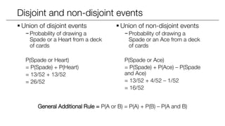
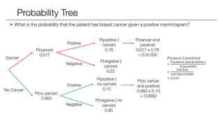
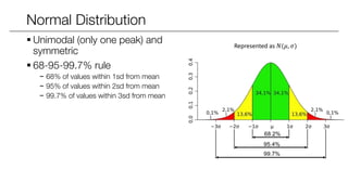
 Expected Mean
𝐸 𝑋
= E[𝑋 × 𝑝 𝑥 ] # sum of all values of x multiplied by its probability
 What is the expected value of a dice roll?
𝐸 𝑋
= 1 ×
1
6
+ 2 ×
1
6
+ 3 ×
1
6
+ 4 ×
1
6
+ 5 ×
1
6
+ 6 ×
1
6
= 3.5
Notation:
𝑥 : sample mean
𝜇 : population mean

10. Mean
 Mean
𝑀𝑒𝑎𝑛
=
𝑥1+ 𝑥2+ 𝑥3+ …+ 𝑥 𝑛
𝑛
 What is the mean number of dots on each die face?
𝑀𝑒𝑎𝑛
=
1+2+3+4+5+6
6
= 3.5
Notation:
𝑥 : sample mean
𝜇 : population mean

11. Expected Variance
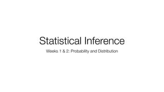
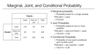
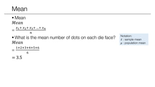
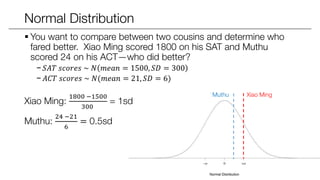
 Expected Variance
𝑉𝑎𝑟 𝑋
=E[(𝑋 − 𝜇)2] # sum square of difference between each value and mean
=E 𝑋2 − 𝐸[𝑋]2
 What is the variance of a dice roll?
From previous slide, mean 𝐸 𝑋 = 3.5
𝐸 𝑋2 = 12 ×
1
6
+ 22 ×
1
6
+ 32 ×
1
6
+ 42 ×
1
6
+ 52 ×
1
6
+ 62 ×
1
6
= 15.17
Var(X) = 𝐸 𝑋2 − 𝐸 𝑋 2 = 15.17 − 3.52 ≈ 2.9
Notation:
𝑠2: sample variance
𝜎2
: population variance
𝑠 : sample standard deviation
𝜎 : population standard deviation

12. Population Variance
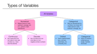
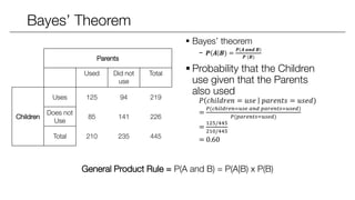
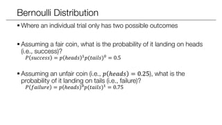
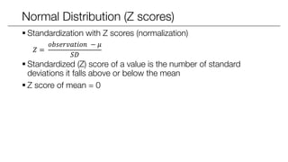
 Population Variance
𝜎2
=
1
𝑁
Σ[(𝑥𝑖 − 𝜇)2
]
 What is the variance of dots on die faces?
Given 𝑥 = 3.5
𝜎2 =
1
6
[ 1 − 3.5 2 + 2 − 3.5 2 + … + 6 − 3.5 2]
≈ 2.9
Notation:
𝑠2: sample variance
𝜎2
: population variance
𝑠 : sample standard deviation
𝜎 : population standard deviation

13. Sample Variance
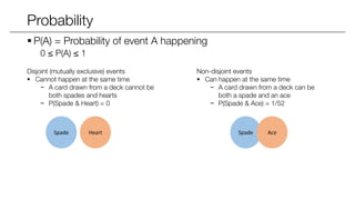
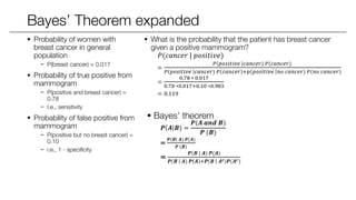
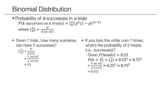
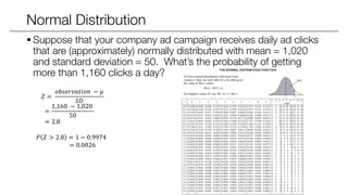
 Sample Variance
𝑠2
=
1
𝑛−1
Σ[(𝑥𝑖 − 𝑥)2
]
 Why n – 1?
− A sample will always have smaller variance than the population. Thus, we
perform an “adjustment” to get a bigger variance that more closer
approximates the population variance
− i.e., think of it as a “correction” used on samples
Notation:
𝑠2: sample variance
𝜎2
: population variance
𝑠 : sample standard deviation
𝜎 : population standard deviation

14. Bernoulli Distribution
 Where an individual trial only has two possible outcomes
 Assuming a fair coin, what is the probability of it landing on heads
(i.e., success)?
𝑃 𝑠𝑢𝑐𝑐𝑒𝑠𝑠 = 𝑝 ℎ𝑒𝑎𝑑𝑠 1
𝑝(𝑡𝑎𝑖𝑙𝑠)0
= 0.5
 Assuming an unfair coin (i.e., 𝑝 ℎ𝑒𝑎𝑑𝑠 = 0.25), what is the
probability of it landing on tails (i.e., failure)?
𝑃 𝑓𝑎𝑖𝑙𝑢𝑟𝑒 = 𝑝 ℎ𝑒𝑎𝑑𝑠 0
𝑝(𝑡𝑎𝑖𝑙𝑠)1
= 0.75

15. Binomial Distribution
 Probability of k successes in n trials
𝑃 𝑘 𝑠𝑢𝑐𝑐𝑒𝑠𝑠𝑒𝑠 𝑖𝑛 𝑛 𝑡𝑟𝑖𝑎𝑙𝑠 = ( 𝑘
𝑛
) 𝑝 𝑘(1 − 𝑝)(𝑛−𝑘)
where ( 𝑘
𝑛
) =
𝑛!
𝑘! 𝑛−𝑘 !
 Given 7 trials, how many scenarios
can have 2 successes?
(2
7
) =
7!
2!(5!)
=
7 ×6 ×5!
2 ×1×5!
= 21
 If you toss the unfair coin 7 times,
what’s the probability of 2 heads
(i.e., successes)?
Given 𝑃 ℎ𝑒𝑎𝑑𝑠 = 0.25
𝑃 𝑘 = 2 = (2
7
) × 0.252 × 0.755
=
7 ×6 ×5!
2 ×1×5!
× 0.252 × 0.755
= 0.311

16. Normal Distribution
 Unimodal (only one peak) and
symmetric
 68-95-99.7% rule
− 68% of values within 1sd from mean
− 95% of values within 2sd from mean
− 99.7% of values within 3sd from mean
Represented as 𝑁(𝜇, 𝜎)

17. Xiao MingMuthu
Normal Distribution
 You want to compare between two cousins and determine who
fared better. Xiao Ming scored 1800 on his SAT and Muthu
scored 24 on his ACT—who did better?
− 𝑆𝐴𝑇 𝑠𝑐𝑜𝑟𝑒𝑠 ~ 𝑁 𝑚𝑒𝑎𝑛 = 1500, 𝑆𝐷 = 300
− 𝐴𝐶𝑇 𝑠𝑐𝑜𝑟𝑒𝑠 ~ 𝑁(𝑚𝑒𝑎𝑛 = 21, 𝑆𝐷 = 6)
Xiao Ming:
1800 −1500
300
= 1sd
Muthu:
24 −21
6
= 0.5sd

18. Normal Distribution (Z scores)
 Standardization with Z scores (normalization)
𝑍 =
𝑜𝑏𝑠𝑒𝑟𝑣𝑎𝑡𝑖𝑜𝑛 − 𝜇
𝑆𝐷
 Standardized (Z) score of a value is the number of standard
deviations it falls above or below the mean
 Z score of mean = 0

19. Normal Distribution
 Suppose that your company ad campaign receives daily ad clicks
that are (approximately) normally distributed with mean = 1,020
and standard deviation = 50. What’s the probability of getting
more than 1,160 clicks a day?
𝑍 =
𝑜𝑏𝑠𝑒𝑟𝑣𝑎𝑡𝑖𝑜𝑛 − 𝜇
𝑆𝐷
=
1,160 − 1,020
50
= 2.8
𝑃 𝑍 > 2.8 = 1 − 0.9974
= 0.0026

20. Normal Distribution
 Your friend boast that his ad is in the top 25% of the company’s
ad campaign. What is the lowest number of ad clicks his ad
received?
− 𝐴𝑑 𝑐𝑙𝑖𝑐𝑘𝑠 ~ 𝑁(1020, 50)
𝑍 = 0.67 =
𝑥 − 1,020
50
𝑥 = 0.67 × 50 + 1020
= 1053.5

21. Poisson Distribution
 Poisson Distribution
𝑃 𝑋 =
𝑒−𝜆 𝜆 𝑥
𝑥!
− 𝑒 = 𝑏𝑎𝑠𝑒 𝑜𝑓 𝑛𝑎𝑡𝑢𝑟𝑎𝑙 𝑙𝑜𝑔, 2.71828 …
− 𝜆 = 𝑚𝑒𝑎𝑛 𝑛𝑢𝑚𝑏𝑒𝑟 𝑜𝑓 𝑠𝑢𝑐𝑐𝑒𝑠𝑠𝑒𝑠 𝑖𝑛 𝑎 𝑔𝑖𝑣𝑒𝑛 𝑡𝑖𝑚𝑒 𝑖𝑛𝑡𝑒𝑟𝑣𝑎𝑙
 2.5 people show up at a bus stop every hour. What is the
probability that 3 or fewer people show up after 4 hours?
𝑃 𝑋 ≤ 3 =
𝑒−10100
0!
+
𝑒−10101
1!
+
𝑒−10102
2!
+
𝑒−10103
3!
= 0.10336

22. Thank you for your attention!
Eugene Yan