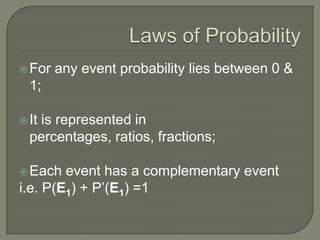
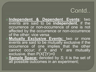
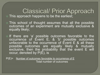
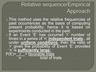
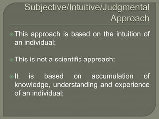
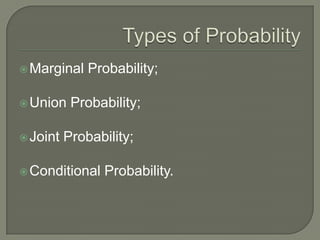
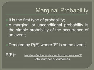
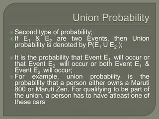
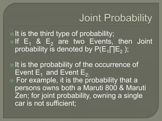
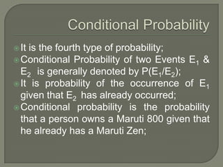
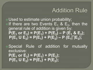
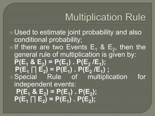
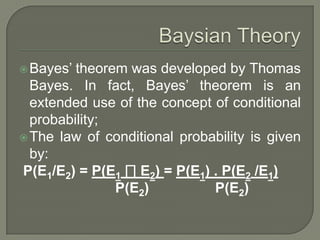
This document discusses key concepts in probability theory including: - Probability is a quantitative measure of uncertainty ranging from 0 to 1. - Experiments produce outcomes that define events in a sample space. - There are different approaches to determining probability (classical, relative frequency, subjective). - Probability can be classified as marginal, union, joint, or conditional depending on the relationship between events. 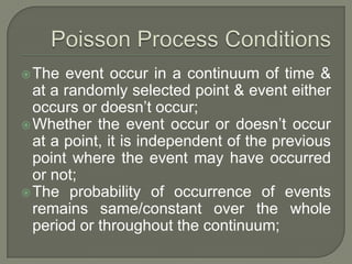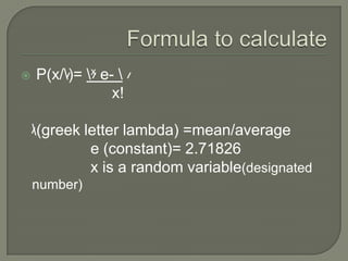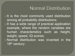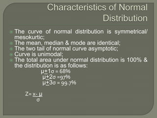- Common discrete and continuous probability distributions include the binomial, Poisson, and normal distributions.

1. Unit IV

2.  Probability is the likelihood or chance that
a particular event will or will not occur;
The theory of probability provides a
quantitative measure of uncertainty of
occurrence of different events resulting
from a random experiment, in terms of
quantitative measures ranging from 0 to 1;

3.  Experiment: it is a process which produces
outcomes; Example, tossing a coin is an
experiment; an interview to gauge the job
satisfaction levels of the employees in an
organization is an experiment;
 Event: it is the outcome of an experiment;
Example, if the experiment is to toss a fair
coin, an event can be obtaining a head; if an
event has a single possible outcome, then it
is a simple (or elementary) event; a subset of
outcomes corresponding to a specific event is
called an event space.

4.  Independent & Dependent Events: two
events are said to be independent, if the
occurrence or non-occurrence of one is not
affected by the occurrence or non-occurrence
of the other; vice versa
 Mutually Exclusive Events: two or more
events are said to be mutually exclusive if the
occurrence of one implies that the other
cannot occur; if X and Y are mutually
exclusive, then P(X∏Y)=0
 Sample Space: denoted by S; it is the set of
all possible outcomes in an experiment;

5. Classical/ Prior Approach;
Relative sequence/Empirical Approach;&
Subjective/Intuitive/Judgmental Approach.

6.  This approach happens to be the earliest;
 This school of thought assumes that all the possible
outcomes of an experiment are mutually exclusive &
equally likely;
 If there are ‘a’ possible outcomes favorable to the
occurrence of Event E, & ‘b’ possible outcomes
unfavorable to the occurrence of Event E & all these
possible outcomes are equally likely & mutually
exclusive, then the probability that the event E will
occur, denoted by P(E), is
P(E)= Number of outcomes favorable to occurrence of E
Total number of outcomes

7. This approach has two characteristics:
a. The subjects refers to fair coins, fair
decks of cards; but if the coin is
unbalanced or there is a loaded dice, this
approach would offer nothing but
confusion;
b. In order to determine probabilities, no
coins had to be tossed, no cards
shuffled, i.e. no experimental data were
required to be collected;

8.  This method uses the relative frequencies of
past occurrences as the basis of computing
present probability; hence it is based on
experiments conducted in the past;
 If an Event ‘E’ has occurred ‘r’ number of
times in a series of ‘n’ independent trials;, all
under uniform conditions, then the ratio of
‘r’ gives the probability of Event ‘E’ provided
‘n’ is sufficiently large:
P(E)= r = favorable trials
n total of trials

9. This approach is based on the intuition of
an individual;
This is not a scientific approach;
It is based on accumulation of
knowledge, understanding and experience
of an individual;

10. For any event probability lies between 0 &
1;
It is represented in
percentages, ratios, fractions;
Each event has a complementary event
i.e. P(E1) + P’(E1) =1

11. Marginal Probability;
Union Probability;
Joint Probability;
Conditional Probability.

12. It is the first type of probability;
A marginal or unconditional probability is
the simple probability of the occurrence of
an event;
Denoted by P(E) where ‘E’ is some event;
P(E)= Number of outcomes favorable to occurrence of E
Total number of outcomes

13.  Second type of probability;
 If E1 & E2 are two Events, then Union
probability is denoted by P(E1 U E2 );
 It is the probability that Event E1 will occur or
that Event E2 will occur or both Event E1 &
Event E2 will occur;
 For example, union probability is the
probability that a person either owns a Maruti
800 or Maruti Zen. For qualifying to be part of
the union, a person has to have atleast one of
these cars

14. It is the third type of probability;
If E1 & E2 are two Events, then Joint
probability is denoted by P(E1∏E2 );
It is the probability of the occurrence of
Event E1 and Event E2;
 For example, it is the probability that a
persons owns both a Maruti 800 & Maruti
Zen; for joint probability, owning a single
car is not sufficient;

15. It is the fourth type of probability;
Conditional Probability of two Events E1 &
E2 is generally denoted by P(E1/E2);
It is probability of the occurrence of E1
given that E2 has already occurred;
Conditional probability is the probability
that a person owns a Maruti 800 given that
he already has a Maruti Zen;

16. Used to estimate union probability;
If there are two Events E1 & E2, then the
general rule of addition is given by:
P(E1 or E2) = P(E1) + P(E2) – P (E1 & E2);
P(E1 U E2) = P(E1) + P(E2) – P (E1∏E2);
Special Rule of addition for mutually
exclusive:
P(E1 or E2) = P(E1) + P(E2);
P(E1 U E2) = P(E1) + P(E2);

17. Used to estimate joint probability and also
conditional probability;
If there are two Events E1 & E2, then the
general rule of multiplication is given by:
P(E1 & E2) = P(E1) . P(E2 /E1);
P(E1 ∏ E2) = P(E1) . P(E2 /E1) ;
Special Rule of multiplication for
independent events:
P(E1 & E2) = P(E1) . P(E2);
P(E1 ∏ E2) = P(E1) . P(E2);

18. Bayes’ theorem was developed by Thomas
Bayes. In fact, Bayes’ theorem is an
extended use of the concept of conditional
probability;
The law of conditional probability is given
by:
P(E1/E2) = P(E1 ∏ E2) = P(E1) . P(E2 /E1)
P(E2) P(E2)

20.  A random variable is a variable which
contains the outcome of a chance
experiment; for example, in an experiment to
measure the number of customers who arrive
in a shop during a time interval of 2 minutes;
the possible outcome may vary from 0 to n
customers; these outcomes (0,1,2,3,4,…n)are
the values of the random variable.
 These random variables are called discrete
random variables

21.  In other words , a random variable which assumes
either a finite number of values or a countable infinite
number of possible values is termed as Discrete
Random variable
 On the other hand, random variables that assumes any
numerical value in an interval or can take values at
every point in a given interval is called continuous
random variable. For example, temperatures recorded
for a particular city can assume any number like 32O
F, 32.5O F 35.8O F
 Experiment outcomes which are based on
measurement scale such as time, distance, weight &
temperature can be explained by Continuous Random
variable

22.  Most commonly used & widely known distribution
among all discrete distributions.
 It is a sequence of repeated trials, called Bernoulli
Process which is characterized by:
1. Only two mutually exclusive outcomes are
possible;( one is referred to as success & the
other as failure)
2. The outcomes in a series of trials/observation
constitute independent events;
3. Probability of success (p) or failure (q) is constant
over a number of trials;
4. The number of events is discrete & can be
represented by integers(0,1,2,3,4,onwards)

23. P(X)= nCxpxqn-x
where
n= total number of trials
x = Designated value
p= probability of success
q= probability of failure
nCx= n!___
x!(n-x)!

24.  It is named after the famous French
Mathematician Simeon Poisson;
 It is also a discrete distribution; but there are
a few differences between Binomial &
Poisson distributions. For a given number of
trials the binomial distribution describes a
distribution of two possible outcomes: either
success or failure whereas Poisson focuses
on the number of discrete occurrences over
an interval.
 It is widely used in the field of managerial
decision making; widely used in queuing
models

25. The event occur in a continuum of time &
at a randomly selected point & event either
occurs or doesn’t occur;
Whether the event occur or doesn’t occur
at a point, it is independent of the previous
point where the event may have occurred
or not;
The probability of occurrence of events
remains same/constant over the whole
period or throughout the continuum;

26.  P(x/)= x e-
x!
(greek letter lambda) =mean/average
e (constant)= 2.71826
x is a random variable(designated
number)

27. It is the most commonly used distribution
among all probability distributions;
It has a wide range of practical application
example, where the random variables are
human characteristics such as height,
weight, speed, IQ scores;
Normal distribution was invented in the
18th century;

28.  The curve of normal distribution is symmetrical/
mesokurtic;
 The mean, median & mode are identical;
 The two tail of normal curve asymptotic;
 Curve is unimodal;
 The total area under normal distribution is 100% &
the distribution is as follows:
µ+1σ = 68%
µ+2σ =97%
µ+3σ = 99.7%
Z= x- µ
σ