This document provides an overview of teaching basic probability and probability distributions to tertiary level teachers. It introduces key concepts such as random experiments, sample spaces, events, assigning probabilities, conditional probability, independent events, and random variables. Examples are provided for each concept to illustrate the definitions and computations. The goal is to explain the necessary probability foundations for teachers to understand sampling distributions and assessing the reliability of statistical estimates from samples.
![Session 2.2
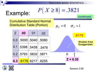
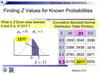
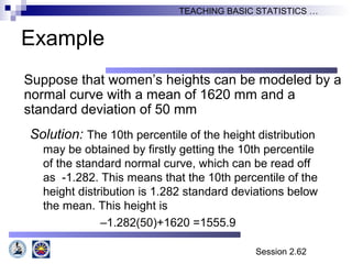
TEACHING BASIC STATISTICS …
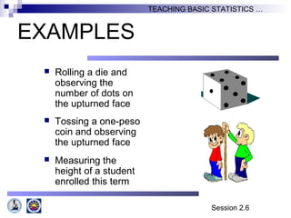
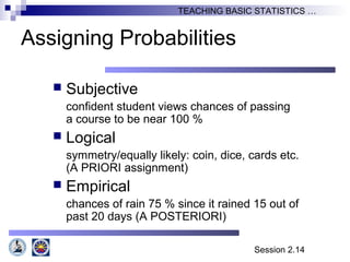
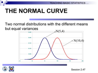
Motivation for Studying Chance
Sample Statistic Estimates Population Parameter
e.g. Sample Mean X = 50 estimates Population Mean µ
Questions:
1. How do we assess the reliability of our estimate?
2. What is an adequate sample size? [ We would expect a
large sample to give better estimates. Large samples
more costly.]](https://image.slidesharecdn.com/session2probability-181231025204/85/Introduction-to-Probability-and-Probability-Distributions-2-320.jpg)
![Session 2.18
TEACHING BASIC STATISTICS …
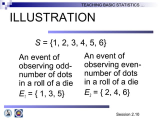
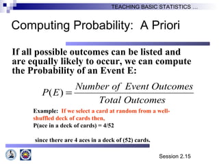
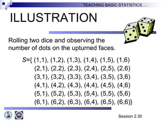
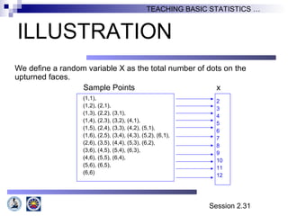
ILLUSTRATION
Suppose the experiment was done for
100 times and it was observed that an
odd-number of dots occurred 60 times
and even-number of dots occurred 40
times.
The (empirical) probability of an event
of observing odd-number of dots in a
roll of a die is the relative frequency of
the event or P[E1] = 60/100 = 0.6](https://image.slidesharecdn.com/session2probability-181231025204/85/Introduction-to-Probability-and-Probability-Distributions-18-320.jpg)
![Session 2.27
TEACHING BASIC STATISTICS …
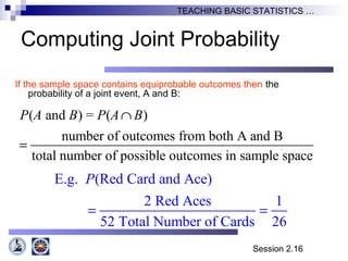
UNEQUALLY LIKELY OUTCOME
ASSUMPTION
The outcomes have different
likelihood to occur.
The probability of an event E is
then computed as the sum of the
probabilities of the outcomes
found in the event E, that is,
P[E] = sum of p{e}
where e is an element of event E.](https://image.slidesharecdn.com/session2probability-181231025204/85/Introduction-to-Probability-and-Probability-Distributions-26-320.jpg)
![Session 2.28
TEACHING BASIC STATISTICS …
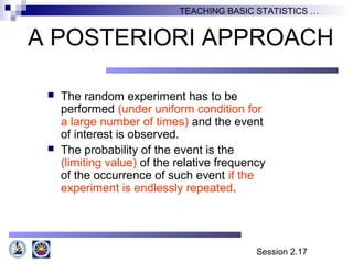
ILLUSTRATION
S = {1, 2, 3, 4, 5, 6}
Assuming that the probability of each of the
outcomes 1,2, and 3 is 1/12 while each of the
outcomes 4, 5 and 6 has likelihood to occur equal
to 1/4.
The probability of an event of observing odd-
number of dots in a roll of a die is P[E1] = sum of
p{1}, p{3} and p{5} = 1/12 + 1/12 + 1/4 = 5/12.](https://image.slidesharecdn.com/session2probability-181231025204/85/Introduction-to-Probability-and-Probability-Distributions-27-320.jpg)
![Session 2.35
TEACHING BASIC STATISTICS …
ILLUSTRATION
The probability distribution of the random variable, X defined
as the total number of dots on the upturned faces in a roll of
two dice, is presented as a table below:
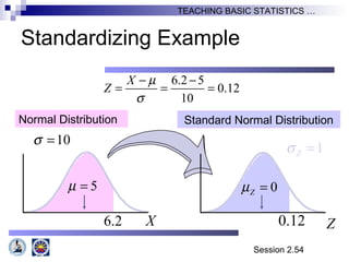
X 2 3 4 5 6 7 8 9 10 11 12
P[X=x] 1/36 2/36 3/36 4/36 5/36 6/36 5/36 4/36 3/36 2/36 1/36
0.00
0.05
0.10
0.15
0.20
2 3 4 5 6 7 8 9 10 11 12
X = Total Number of Dots on the Upturned faces](https://image.slidesharecdn.com/session2probability-181231025204/85/Introduction-to-Probability-and-Probability-Distributions-34-320.jpg)
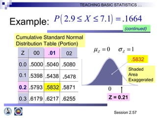
![Session 2.53
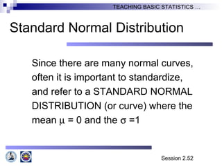
TEACHING BASIC STATISTICS …
THE Z-TABLE
P[Z ≤ z]
Examples:
1. P[Z ≤ 0] = 0.5
2. P[Z ≤ 1.25] = 0.8944
3. P[Z ≤ 1.96] = 0.9750
0 z
This table summarizes the cumulative probability
distribution for Z (i.e. P[Z ≤ z])](https://image.slidesharecdn.com/session2probability-181231025204/85/Introduction-to-Probability-and-Probability-Distributions-52-320.jpg)
![Session 2.63
TEACHING BASIC STATISTICS …
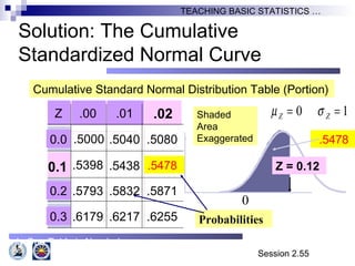
RULES IN COMPUTING PROBABILITIES
P[Z = a] = 0
P[Z ≤ a] can be obtained directly
from the Z-table
P[Z ≥ a] = 1 – P[Z ≤ a]
P[Z ≥ -a] = P[Z ≤ +a]
P[Z ≤ -a] = P[Z ≥ +a]
P[a1 ≤ Z ≤ a2] = P[Z ≤ a2] – P[Z ≤ a1]](https://image.slidesharecdn.com/session2probability-181231025204/85/Introduction-to-Probability-and-Probability-Distributions-62-320.jpg)


![[DSC Europe 25] Ivan Lukovic & Marija Djukic - From Data to Value: Why Maturi...](https://cdn.slidesharecdn.com/ss_thumbnails/ahrfps8xr6knowwhacxh-1-ivan-marija-dsc-2025-ld-v1-presentation-260115093812-be21adfc-thumbnail.jpg?width=640&height=640&fit=bounds)