This document discusses various probability distributions including discrete and continuous distributions. It covers the binomial, hypergeometric, Poisson, and normal distributions. For each distribution, it provides the characteristics and formulas, and examples of how to calculate probabilities using the distributions and probability tables or software. It also illustrates how the parameters impact the shape of the distributions. The goal is to help readers apply different probability distributions to problems and compute probabilities.

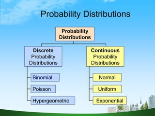
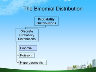
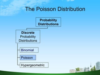
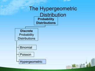
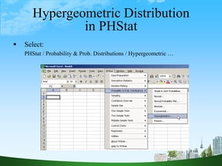
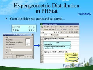
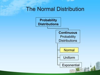
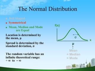
1. 1
Discrete and Continuous
Probability Distributions

2. 2
Chapter Goals
After completing this chapter, you should be
able to:
 Apply the binomial distribution to applied
problems
 Compute probabilities for the Poisson and
hypergeometric distributions
 Find probabilities using a normal distribution
table and apply the normal distribution to
business problems
 Recognize when to apply the uniform and

3. 3
Probability Distributions
Continuous
Probability
Distributions
Binomial
Hypergeometric
Poisson
Probability
Distributions
Discrete
Probability
Distributions
Normal
Uniform
Exponential

4. 4
 A discrete random variable is a variable that
can assume only a countable number of values
Many possible outcomes:
 number of complaints per day
 number of TV’s in a household
 number of rings before the phone is answered
Only two possible outcomes:
 gender: male or female
 defective: yes or no
 spreads peanut butter first vs. spreads jelly first
Discrete Probability Distributions

5. 5
Continuous Probability Distributions
 A continuous random variable is a variable
that can assume any value on a continuum
(can assume an uncountable number of
values)
 thickness of an item
 time required to complete a task
 temperature of a solution
 height, in inches
 These can potentially take on any value,
depending only on the ability to measure

6. 6
The Binomial Distribution
Binomial
Hypergeometric
Poisson
Probability
Distributions
Discrete
Probability
Distributions

7. 7
The Binomial Distribution
 Characteristics of the Binomial Distribution:
 A trial has only two possible outcomes – “success” or
“failure”
 There is a fixed number, n, of identical trials
 The trials of the experiment are independent of each other
 The probability of a success, p, remains constant from trial to
trial
 If p represents the probability of a success, then
(1-p) = q is the probability of a failure

8. 8
Binomial Distribution Settings
 A manufacturing plant labels items as either
defective or acceptable
 A firm bidding for a contract will either get the
contract or not
 A marketing research firm receives survey
responses of “yes I will buy” or “no I will not”
 New job applicants either accept the offer or
reject it

9. 9
Counting Rule for Combinations
 A combination is an outcome of an experiment where
x objects are selected from a group of n objects
)!
x
n
(
!
x
!
n
Cn
x


where:
n! =n(n - 1)(n - 2) . . . (2)(1)
x! = x(x - 1)(x - 2) . . . (2)(1)
0! = 1 (by definition)

10. 10
P(x) = probability of x successes in n trials,
with probability of success p on each trial
x = number of ‘successes’ in sample,
(x = 0, 1, 2, ..., n)
p = probability of “success” per trial
q = probability of “failure” = (1 – p)
n = number of trials (sample size)
P(x)
n
x ! n x
p q
x n x
!
( )!



Example: Flip a coin four
times, let x = # heads:
n = 4
p = 0.5
q = (1 - .5) = .5
x = 0, 1, 2, 3, 4
Binomial Distribution Formula

11. 11
n = 5 p = 0.1
n = 5 p = 0.5
Mean
0
.2
.4
.6
0 1 2 3 4 5
X
P(X)
.2
.4
.6
0 1 2 3 4 5
X
P(X)
0
Binomial Distribution
 The shape of the binomial
distribution depends on the
values of p and n
Here, n = 5 and p = .1
Here, n = 5 and p = .5

12. 12
Binomial Distribution
Characteristics
 Mean
Variance and Standard Deviation
np
E(x)
μ 

npq
σ
2

npq
σ
Where n = sample size
p = probability of success
q = (1 – p) = probability of failure

13. 13
n = 5 p = 0.1
n = 5 p = 0.5
Mean
0
.2
.4
.6
0 1 2 3 4 5
X
P(X)
.2
.4
.6
0 1 2 3 4 5
X
P(X)
0
0.5
(5)(.1)
np
μ 


0.6708
.1)
(5)(.1)(1
npq
σ




2.5
(5)(.5)
np
μ 


1.118
.5)
(5)(.5)(1
npq
σ




Binomial Characteristics
Examples

14. 14
Using Binomial Tables
n = 10
x p=.15 p=.20 p=.25 p=.30 p=.35 p=.40 p=.45 p=.50
0
1
2
3
4
5
6
7
8
9
10
0.1969
0.3474
0.2759
0.1298
0.0401
0.0085
0.0012
0.0001
0.0000
0.0000
0.0000
0.1074
0.2684
0.3020
0.2013
0.0881
0.0264
0.0055
0.0008
0.0001
0.0000
0.0000
0.0563
0.1877
0.2816
0.2503
0.1460
0.0584
0.0162
0.0031
0.0004
0.0000
0.0000
0.0282
0.1211
0.2335
0.2668
0.2001
0.1029
0.0368
0.0090
0.0014
0.0001
0.0000
0.0135
0.0725
0.1757
0.2522
0.2377
0.1536
0.0689
0.0212
0.0043
0.0005
0.0000
0.0060
0.0403
0.1209
0.2150
0.2508
0.2007
0.1115
0.0425
0.0106
0.0016
0.0001
0.0025
0.0207
0.0763
0.1665
0.2384
0.2340
0.1596
0.0746
0.0229
0.0042
0.0003
0.0010
0.0098
0.0439
0.1172
0.2051
0.2461
0.2051
0.1172
0.0439
0.0098
0.0010
10
9
8
7
6
5
4
3
2
1
0
p=.85 p=.80 p=.75 p=.70 p=.65 p=.60 p=.55 p=.50 x
Examples:
n = 10, p = .35, x = 3: P(x = 3|n =10, p = .35) = .2522
n = 10, p = .75, x = 2: P(x = 2|n =10, p = .75) = .0004

15. 15
Using PHStat
 Select PHStat / Probability & Prob. Distributions / Binomial…

16. 16
Using PHStat
 Enter desired values in dialog box
Here: n = 10
p = .35
Output for x = 0
to x = 10 will be
generated by PHStat
Optional check boxes
for additional output

17. 17
P(x = 3 | n = 10, p = .35) = .2522
PHStat Output
P(x > 5 | n = 10, p = .35) = .0949

18. 18
The Poisson Distribution
Binomial
Hypergeometric
Poisson
Probability
Distributions
Discrete
Probability
Distributions

19. 19
The Poisson Distribution
 Characteristics of the Poisson Distribution:
 The outcomes of interest are rare relative to the
possible outcomes
 The average number of outcomes of interest per
time or space interval is 
 The number of outcomes of interest are random,
and the occurrence of one outcome does not
influence the chances of another outcome of
interest
 The probability of that an outcome of interest
occurs in a given segment is the same for all

20. 20
Poisson Distribution Formula
where:
t = size of the segment of interest
x = number of successes in segment of interest
 = expected number of successes in a segment of unit size
e = base of the natural logarithm system (2.71828...)
!
x
e
)
t
(
)
x
(
P
t
x 




21. 21
Poisson Distribution Characteristics
 Mean
Variance and Standard Deviation
λt
μ 
λt
σ2

λt
σ
where  = number of successes in a segment of unit size
t = the size of the segment of interest

22. 22
Using Poisson Tables
X
t
0.10 0.20 0.30 0.40 0.50 0.60 0.70 0.80 0.90
0
1
2
3
4
5
6
7
0.9048
0.0905
0.0045
0.0002
0.0000
0.0000
0.0000
0.0000
0.8187
0.1637
0.0164
0.0011
0.0001
0.0000
0.0000
0.0000
0.7408
0.2222
0.0333
0.0033
0.0003
0.0000
0.0000
0.0000
0.6703
0.2681
0.0536
0.0072
0.0007
0.0001
0.0000
0.0000
0.6065
0.3033
0.0758
0.0126
0.0016
0.0002
0.0000
0.0000
0.5488
0.3293
0.0988
0.0198
0.0030
0.0004
0.0000
0.0000
0.4966
0.3476
0.1217
0.0284
0.0050
0.0007
0.0001
0.0000
0.4493
0.3595
0.1438
0.0383
0.0077
0.0012
0.0002
0.0000
0.4066
0.3659
0.1647
0.0494
0.0111
0.0020
0.0003
0.0000
Example: Find P(x = 2) if  = .05 and t = 100
.075
2!
e
(0.50)
!
x
e
)
t
(
)
2
x
(
P
0.50
2
t
x









23. 23
Graph of Poisson Probabilities
0.00
0.10
0.20
0.30
0.40
0.50
0.60
0.70
0 1 2 3 4 5 6 7
x
P(x)
X
t =
0.50
0
1
2
3
4
5
6
7
0.6065
0.3033
0.0758
0.0126
0.0016
0.0002
0.0000
0.0000
P(x = 2) = .0758
Graphically:
 = .05 and t = 100

24. 24
Poisson Distribution Shape
 The shape of the Poisson Distribution depends
on the parameters  and t:
0.00
0.05
0.10
0.15
0.20
0.25
1 2 3 4 5 6 7 8 9 10 11 12
x
P(x)
0.00
0.10
0.20
0.30
0.40
0.50
0.60
0.70
0 1 2 3 4 5 6 7
x
P(x)
t = 0.50 t = 3.0

25. 25
The Hypergeometric
Distribution
Binomial
Poisson
Probability
Distributions
Discrete
Probability
Distributions
Hypergeometric

26. 26
The Hypergeometric Distribution
 “n” trials in a sample taken from a finite
population of size N
 Sample taken without replacement
 Trials are dependent
 Concerned with finding the probability of “x”
successes in the sample where there are “X”
successes in the population

27. 27
Hypergeometric Distribution
Formula
N
n
X
x
X
N
x
n
C
C
C
)
x
(
P



.
Where
N = Population size
X = number of successes in the population
n = sample size
x = number of successes in the sample
n – x = number of failures in the sample
(Two possible outcomes per trial)

28. 28
Hypergeometric Distribution
Formula
0.3
120
(6)(6
C
C
C
C
C
C
2)
P(x 10
3
4
2
6
1
N
n
X
x
X
N
x
n







■ Example: 3 Light bulbs were selected from 10. Of the 10
there were 4 defective. What is the probability that 2 of the 3
selected are defective?
N = 10 n = 3
X = 4 x = 2

29. 29
Hypergeometric Distribution
in PHStat
 Select:
PHStat / Probability & Prob. Distributions / Hypergeometric …

30. 30
Hypergeometric Distribution
in PHStat
 Complete dialog box entries and get output …
N = 10 n = 3
X = 4 x = 2
P(x = 2) = 0.3
(continued)

31. 31
The Normal Distribution
Continuous
Probability
Distributions
Probability
Distributions
Normal
Uniform
Exponential

32. 32
The Normal Distribution
 ‘Bell Shaped’
 Symmetrical
 Mean, Median and Mode
are Equal
Location is determined by
the mean, μ
Spread is determined by the
standard deviation, σ
The random variable has an
infinite theoretical range:
+  to  
Mean
= Median
= Mode
x
f(x)
μ
σ

33. 33
By varying the parameters μ and σ, we obtain
different normal distributions
Many Normal Distributions

34. 34
The Normal Distribution Shape
x
f(x)
μ
σ
Changing μ shifts the
distribution left or right.
Changing σ increases
or decreases the
spread.

35. 35
Finding Normal Probabilities
Probability is the
area under the
curve!
a b x
f(x) P a x b
( )
 
Probability is measured by the area
under the curve

36. 36
f(x)
x
μ
Probability as
Area Under the Curve
0.5
0.5
The total area under the curve is 1.0, and the curve is
symmetric, so half is above the mean, half is below
1.0
)
x
P( 




0.5
)
x
P(
μ 



0.5
μ)
x
P( 




37. 37
Empirical Rules
μ ± 1σ encloses about 68%
of x’s
f(x)
x
μ μ+1σ
μ1σ
What can we say about the distribution of values
around the mean? There are some general rules:
σ
σ
68.26%

38. 38
The Empirical Rule
 μ ± 2σ covers about 95% of x’s
 μ ± 3σ covers about 99.7% of x’s
x
μ
2σ 2σ
x
μ
3σ 3σ
95.44% 99.72%
(continued)

39. 39
Importance of the Rule
 If a value is about 2 or more standard
deviations away from the mean in a normal
distribution, then it is far from the mean
 The chance that a value that far or farther
away from the mean is highly unlikely, given
that particular mean and standard deviation

40. 40
The Standard Normal Distribution
 Also known as the “z” distribution
 Mean is defined to be 0
 Standard Deviation is 1
z
f(z)
0
1
Values above the mean have positive z-values,
values below the mean have negative z-values

41. 41
The Standard Normal
 Any normal distribution (with any mean and
standard deviation combination) can be
transformed into the standard normal
distribution (z)
 Need to transform x units into z units

42. 42
Translation to the Standard
Normal Distribution
 Translate from x to the standard normal (the
“z” distribution) by subtracting the mean of
x and dividing by its standard deviation:
σ
μ
x
z



43. 43
Example
 If x is distributed normally with mean of
100 and standard deviation of 50, the z
value for x = 250 is
 This says that x = 250 is three standard
deviations (3 increments of 50 units) above
the mean of 100.
3.0
50
100
250
σ
μ
x
z 





44. 44
Comparing x and z units
z
100
3.0
0
250 x
Note that the distribution is the same, only the
scale has changed. We can express the problem in
original units (x) or in standardized units (z)
μ = 100
σ = 50

45. 45
The Standard Normal Table
 The Standard Normal table in the
textbook (Appendix D)
gives the probability from the mean
(zero)
up to a desired value for z
z
0 2.00
.4772
Example:
P(0 < z < 2.00) = .4772

46. 46
The Standard Normal Table
The value within the
table gives the
probability from z = 0
up to the desired z
value
z 0.00 0.01 0.02 …
0.1
0.2
.4772
2.0
P(0 < z < 2.00) = .4772
The row shows
the value of z to
the first decimal
point
The column gives the value of z
to the second decimal point
2.0
.
.
.
(continued)

47. 47
General Procedure for Finding
Probabilities
 Draw the normal curve
for the problem in
terms of x
 Translate x-values to z-
values
 Use the Standard
Normal Table
To find P(a < x < b) when x is distributed
normally:

48. 48
Z Table example
 Suppose x is normal with mean 8.0 and
standard deviation 5.0. Find P(8 < x < 8.6)
P(8 < x < 8.6)
= P(0 < z < 0.12)
Z
0.12
0
x
8.6
8
0
5
8
8
σ
μ
x
z 




0.12
5
8
8.6
σ
μ
x
z 




Calculate z-values:

49. 49
Z Table example
 Suppose x is normal with mean 8.0 and standard
deviation 5.0. Find P(8 < x < 8.6)
P(0 < z < 0.12)
z
0.12
0
x
8.6
8
P(8 < x < 8.6)
 = 8
 = 5
 = 0
 = 1
(continued)

50. 50
Z
0.12
z .00 .01
0.0 .0000 .0040 .0080
.0398 .0438
0.2 .0793 .0832 .0871
0.3 .1179 .1217 .1255
Solution: Finding P(0 < z < 0.12)
.0478
.02
0.1 .0478
Standard Normal Probability
Table (Portion)
0.00
= P(0 < z < 0.12)
P(8 < x < 8.6)

51. 51
Finding Normal Probabilities
 Suppose x is normal with mean 8.0 and
standard deviation 5.0.
 Now Find P(x < 8.6)
Z
8.6
8.0

52. 52
Finding Normal Probabilities
 Suppose x is normal with mean 8.0 and
standard deviation 5.0.
 Now Find P(x < 8.6)
(continued)
Z
0.12
.0478
0.00
.5000
P(x < 8.6)
= P(z < 0.12)
= P(z < 0) + P(0 < z < 0.12)
= .5 + .0478 = .5478

53. 53
Upper Tail Probabilities
 Suppose x is normal with mean 8.0 and
standard deviation 5.0.
 Now Find P(x > 8.6)
Z
8.6
8.0

54. 54
 Now Find P(x > 8.6)…
(continued)
Z
0.12
0
Z
0.12
.0478
0
.5000 .50 - .0478
= .4522
P(x > 8.6) = P(z > 0.12) = P(z > 0) - P(0 < z < 0.12)
= .5 - .0478 = .4522
Upper Tail Probabilities

55. 55
Lower Tail Probabilities
 Suppose x is normal with mean 8.0 and
standard deviation 5.0.
 Now Find P(7.4 < x < 8)
Z
7.4
8.0

56. 56
Lower Tail Probabilities
Now Find P(7.4 < x < 8)…
Z
7.4
8.0
The Normal distribution is
symmetric, so we use the
same table even if z-values
are negative:
P(7.4 < x < 8)
= P(-0.12 < z < 0)
= .0478
(continued)
.0478

57. 57
Normal Probabilities in PHStat
 We can use Excel and PHStat to quickly
generate probabilities for any normal
distribution
 We will find P(8 < x < 8.6) when x is
normally distributed with mean 8 and
standard deviation 5

58. 58
PHStat Dialogue Box
Select desired options
and enter values

59. 59
PHStat Output

60. 60
The Uniform Distribution
Continuous
Probability
Distributions
Probability
Distributions
Normal
Uniform
Exponential

61. 61
The Uniform Distribution
 The uniform distribution is a probability
distribution that has equal probabilities for all
possible outcomes of the random variable

62. 62
The Continuous Uniform Distribution:
otherwise
0
b
x
a
if
a
b
1



where
f(x) = value of the density function at any x value
a = lower limit of the interval
b = upper limit of the interval
The Uniform Distribution (continued)
f(x) =

63. 63
Uniform Distribution
Example: Uniform Probability Distribution
Over the range 2 ≤ x ≤ 6:
2 6
.25
f(x) = = .25 for 2 ≤ x ≤ 6
6 - 2
1
x
f(x)

64. 64
The Exponential Distribution
Continuous
Probability
Distributions
Probability
Distributions
Normal
Uniform
Exponential

65. 65
The Exponential Distribution
 Used to measure the time that elapses between
two occurrences of an event (the time between
arrivals)
 Examples:
 Time between trucks arriving at an unloading dock
 Time between transactions at an ATM Machine
 Time between phone calls to the main operator

66. 66
The Exponential Distribution
a
λ
e
1
a)
x
P(0 




 The probability that an arrival time is equal to or less
than some specified time a is
where 1/ is the mean time between events
Note that if the number of occurrences per time period is Poisson
with mean , then the time between occurrences is exponential
with mean time 1/ 

67. 67
Exponential Distribution
 Shape of the exponential distribution
(continued)
f(x)
x
 = 1.0
(mean = 1.0)
= 0.5
(mean = 2.0)
 = 3.0
(mean = .333)

68. 68
Example
Example: Customers arrive at the claims counter at
the rate of 15 per hour (Poisson distributed). What
is the probability that the arrival time between
consecutive customers is less than five minutes?
 Time between arrivals is exponentially distributed
with mean time between arrivals of 4 minutes (15
per 60 minutes, on average)
 1/ = 4.0, so  = .25
 P(x < 5) = 1 - e-a = 1 – e-(.25)(5) = .7135