Probability_Distributions lessons with random variables
1.
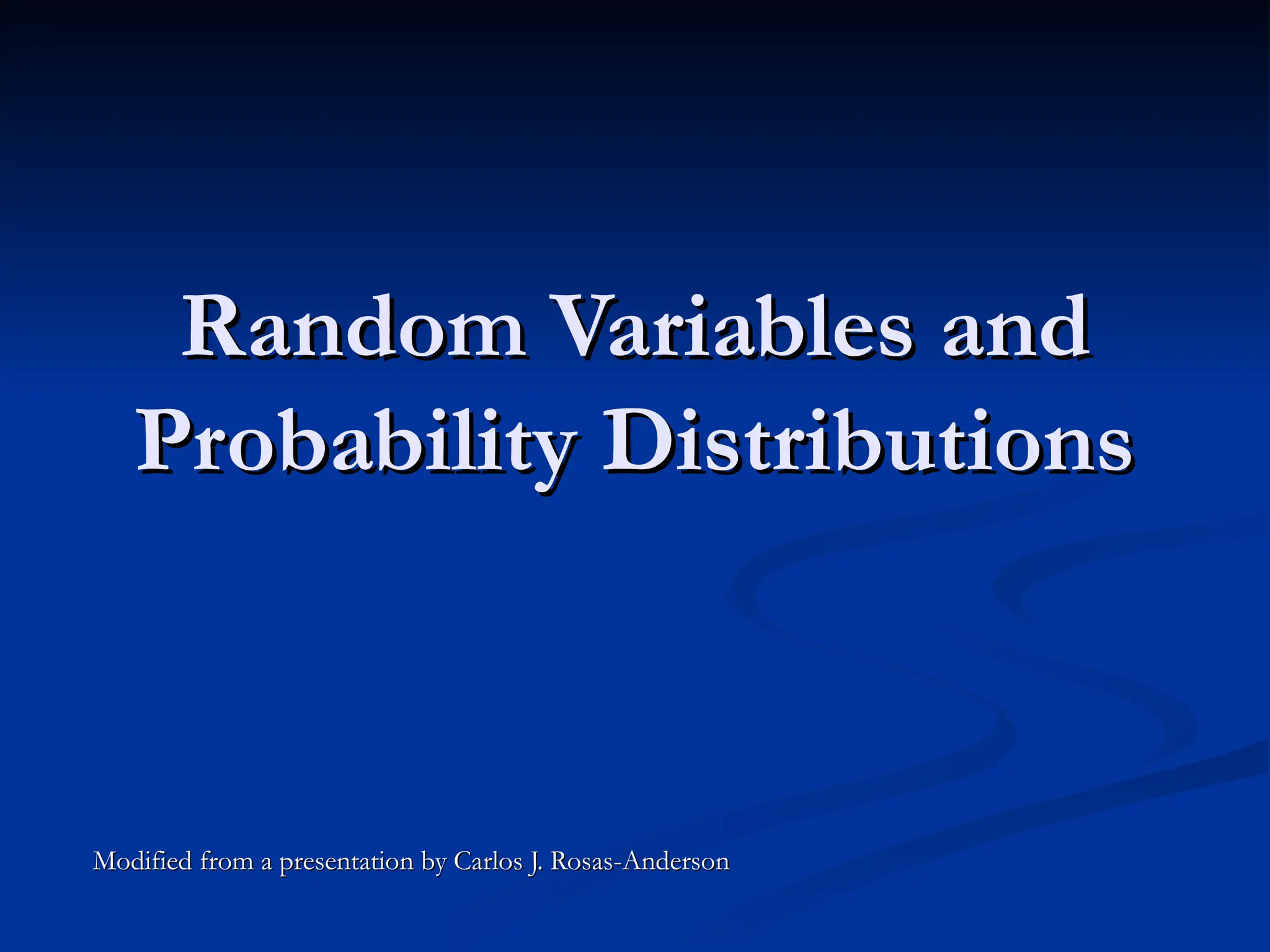
Random Variables and
RandomVariables and
Probability Distributions
Probability Distributions
Modified from a presentation by Carlos J. Rosas-Anderson
Modified from a presentation by Carlos J. Rosas-Anderson
2.
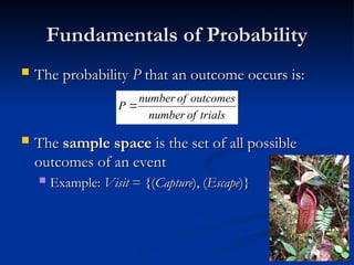
Fundamentals of Probability
Fundamentalsof Probability
The probability
The probability P
P that an outcome occurs is:
that an outcome occurs is:
The
The sample space
sample space is the set of all possible
is the set of all possible
outcomes of an event
outcomes of an event
Example:
Example: Visit
Visit = {(
= {(Capture
Capture), (
), (Escape
Escape)}
)}
trials
of
number
outcomes
of
number
P
3.
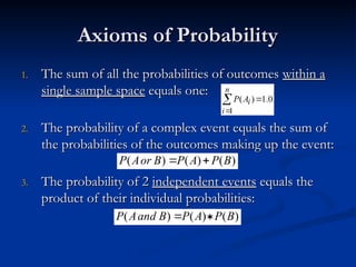
Axioms of Probability
Axiomsof Probability
1.
1. The sum of all the probabilities of outcomes
The sum of all the probabilities of outcomes within a
within a
single sample space
single sample space equals one:
equals one:
2.
2. The probability of a complex event equals the sum of
The probability of a complex event equals the sum of
the probabilities of the outcomes making up the event:
the probabilities of the outcomes making up the event:
3.
3. The probability of 2
The probability of 2 independent events
independent events equals the
equals the
product of their individual probabilities:
product of their individual probabilities:
)
(
)
(
)
( B
P
A
P
B
or
A
P
0
.
1
)
(
1
n
i
i
A
P
)
(
)
(
)
( B
P
A
P
B
and
A
P
4.
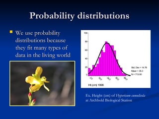
Probability distributions
Probability distributions
We use probability
We use probability
distributions because
distributions because
they fit many types of
they fit many types of
data in the living world
data in the living world
Ht (cm
) 1996
100
80
60
40
20
0
Std. Dev = 14.76
Mean = 35.3
N= 713.00
Ex. Height (cm) of Hypericum cumulicola
at Archbold Biological Station
5.
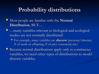
Probability distributions
Probability distributions
Most people are familiar with the
Most people are familiar with the Normal
Normal
Distribution
Distribution, BUT…
, BUT…
…
…many variables relevant to biological and ecological
many variables relevant to biological and ecological
studies are not normally distributed!
studies are not normally distributed!
For example, many variables are
For example, many variables are discrete
discrete (presence/absence,
(presence/absence,
# of seeds or offspring, # of prey consumed, etc.)
# of seeds or offspring, # of prey consumed, etc.)
Because normal distributions apply only to continuous
Because normal distributions apply only to continuous
variables, we need other types of distributions to model
variables, we need other types of distributions to model
discrete variables.
discrete variables.
6.
Random variable
Random variable
The mathematical rule (or function) that
The mathematical rule (or function) that
assigns a given numerical value to each
assigns a given numerical value to each
possible outcome of an experiment in the
possible outcome of an experiment in the
sample space of interest.
sample space of interest.
2 Types:
2 Types:
Discrete random variables
Discrete random variables
Continuous random variables
Continuous random variables
7.
The Binomial Distribution
TheBinomial Distribution
Bernoulli Random Variables
Bernoulli Random Variables
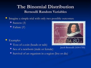
Imagine a simple trial with only two possible outcomes:
Imagine a simple trial with only two possible outcomes:
Success (
Success (S
S)
)
Failure (
Failure (F
F)
)
Examples
Examples
Toss of a coin (heads or tails)
Toss of a coin (heads or tails)
Sex of a newborn (male or female)
Sex of a newborn (male or female)
Survival of an organism in a region (live or die)
Survival of an organism in a region (live or die)
Jacob Bernoulli (1654-1705)
8.
The Binomial Distribution
TheBinomial Distribution
Overview
Overview
Suppose that the probability of success is
Suppose that the probability of success is p
p
What is the probability of failure?
What is the probability of failure?
q
q = 1 –
= 1 – p
p
Examples
Examples
Toss of a coin (
Toss of a coin (S
S = head):
= head): p
p = 0.5
= 0.5
q
q = 0.5
= 0.5
Roll of a die (
Roll of a die (S
S = 1):
= 1): p
p = 0.1667
= 0.1667
q
q = 0.8333
= 0.8333
Fertility of a chicken egg (
Fertility of a chicken egg (S
S = fertile):
= fertile): p
p = 0.8
= 0.8
q
q = 0.2
= 0.2
9.
The Binomial Distribution
TheBinomial Distribution
Overview
Overview
Imagine that a trial is repeated
Imagine that a trial is repeated n
n times
times
Examples:
Examples:
A coin is tossed 5 times
A coin is tossed 5 times
A die is rolled 25 times
A die is rolled 25 times
50 chicken eggs are examined
50 chicken eggs are examined
ASSUMPTIONS:
ASSUMPTIONS:
1)
1) p
p is constant from trial to trial
is constant from trial to trial
2)
2) the trials are statistically independent of each other
the trials are statistically independent of each other
10.
The Binomial Distribution
TheBinomial Distribution
Overview
Overview
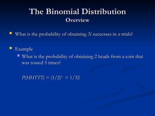
What is the probability of obtaining
What is the probability of obtaining X
X successes in
successes in n
n trials?
trials?
Example
Example
What is the probability of obtaining 2 heads from a coin that
What is the probability of obtaining 2 heads from a coin that
was tossed 5 times?
was tossed 5 times?
P
P(
(HHTTT
HHTTT) = (1/2)
) = (1/2)5
5
= 1/32
= 1/32
11.
The Binomial Distribution
TheBinomial Distribution
Overview
Overview
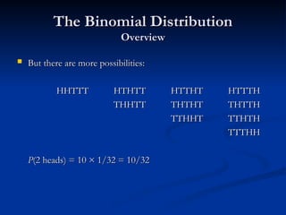
But there are more possibilities:
But there are more possibilities:
HHTTT
HHTTT HTHTT
HTHTT HTTHT
HTTHT HTTTH
HTTTH
THHTT
THHTT THTHT
THTHT THTTH
THTTH
TTHHT
TTHHT TTHTH
TTHTH
TTTHH
TTTHH
P
P(2 heads) = 10 × 1/32 = 10/32
(2 heads) = 10 × 1/32 = 10/32
12.
The Binomial Distribution
TheBinomial Distribution
Overview
Overview
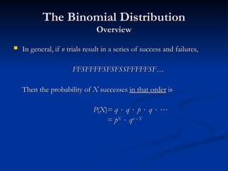
In general, if
In general, if n
n trials result in a series of success and failures,
trials result in a series of success and failures,
FFSFFFFSFSFSSFFFFFSF…
FFSFFFFSFSFSSFFFFFSF…
Then the probability of
Then the probability of X
X successes
successes in that order
in that order is
is
P
P(
(X
X)
)=
= q
q
q
q
p
p
q
q
=
= p
pX
X
q
qn
n –
– X
X
13.
The Binomial Distribution
TheBinomial Distribution
Overview
Overview
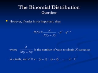
However, if order is not important, then
However, if order is not important, then
where is the number of ways to obtain
where is the number of ways to obtain X
X successes
successes
in
in n
n trials, and
trials, and n
n! =
! = n
n
(
(n
n – 1)
– 1)
(
(n
n – 2)
– 2)
…
…
2
2
1
1
n!
X!(n – X)!
p
pX
X
q
qn – X
n – X
P
P(
(X
X) =
) =
n!
X!(n – X)!
14.
The Binomial Distribution
TheBinomial Distribution
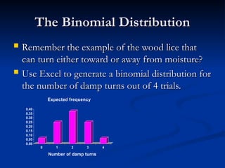
Remember the example of the wood lice that
Remember the example of the wood lice that
can turn either toward or away from moisture?
can turn either toward or away from moisture?
Use Excel to generate a binomial distribution for
Use Excel to generate a binomial distribution for
the number of damp turns out of 4 trials.
the number of damp turns out of 4 trials.
0.00
0.05
0.10
0.15
0.20
0.25
0.30
0.35
0.40
0 1 2 3 4
Number of damp turns
Expected frequency
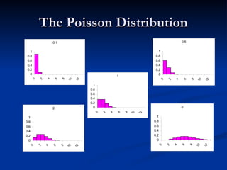
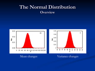
The Poisson Distribution
ThePoisson Distribution
Overview
Overview
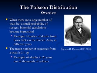
When there are a large number of
When there are a large number of
trials but a small probability of
trials but a small probability of
success, binomial calculations
success, binomial calculations
become impractical
become impractical
Example: Number of deaths from
Example: Number of deaths from
horse kicks in the French Army in
horse kicks in the French Army in
different years
different years
The mean number of successes from
The mean number of successes from
n
n trials is
trials is λ
λ =
= np
np
Example: 64 deaths in 20 years
Example: 64 deaths in 20 years
out of thousands of soldiers
out of thousands of soldiers
Simeon D. Poisson (1781-1840)
17.
The Poisson Distribution
ThePoisson Distribution
Overview
Overview
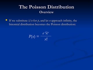
If we substitute
If we substitute λ
λ/
/n
n for
for p
p, and let
, and let n
n approach infinity, the
approach infinity, the
binomial distribution becomes the Poisson distribution:
binomial distribution becomes the Poisson distribution:
P(x) =
e-λ
λx
x!
18.
The Poisson Distribution
ThePoisson Distribution
Overview
Overview
The Poisson distribution is applied when random events are
The Poisson distribution is applied when random events are
expected to occur in a fixed area or a fixed interval of time
expected to occur in a fixed area or a fixed interval of time
Deviation from a Poisson distribution may indicate some degree
Deviation from a Poisson distribution may indicate some degree
of non-randomness in the events under study
of non-randomness in the events under study
See Hurlbert (1990) for some caveats and suggestions for
See Hurlbert (1990) for some caveats and suggestions for
analyzing random spatial distributions using Poisson
analyzing random spatial distributions using Poisson
distributions
distributions
19.
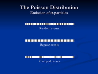
The Poisson Distribution
ThePoisson Distribution
Example: Emission of
Example: Emission of
-particles
-particles
Rutherford, Geiger, and Bateman (1910) counted the number of
Rutherford, Geiger, and Bateman (1910) counted the number of
-particles emitted by a film of polonium in 2608 successive
-particles emitted by a film of polonium in 2608 successive
intervals of one-eighth of a minute
intervals of one-eighth of a minute
What is
What is n
n?
?
What is
What is p
p?
?
Do their data follow a Poisson distribution?
Do their data follow a Poisson distribution?
20.
The Poisson Distribution
ThePoisson Distribution
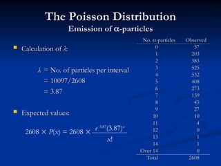
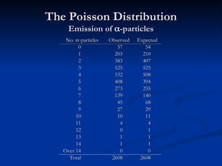
Emission of
Emission of
-particles
-particles
No.
No.
-particles
-particles Observed
Observed
0
0 57
57
1
1 203
203
2
2 383
383
3
3 525
525
4
4 532
532
5
5 408
408
6
6 273
273
7
7 139
139
8
8 45
45
9
9 27
27
10
10 10
10
11
11 4
4
12
12 0
0
13
13 1
1
14
14 1
1
Over 14
Over 14 0
0
Total
Total 2608
2608
Calculation of
Calculation of λ
λ:
:
λ
λ = No. of particles per interval
= No. of particles per interval
= 10097/2608
= 10097/2608
= 3.87
= 3.87
Expected values:
Expected values:
2608 P(x) =
e-3.87
(3.87)x
x!
2608
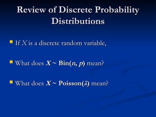
Review of DiscreteProbability
Review of Discrete Probability
Distributions
Distributions
If
If X
X is a discrete random variable,
is a discrete random variable,
What does
What does X
X ~ Bin(
~ Bin(n
n,
, p
p)
) mean?
mean?
What does
What does X
X ~ Poisson(
~ Poisson(λ
λ)
) mean?
mean?
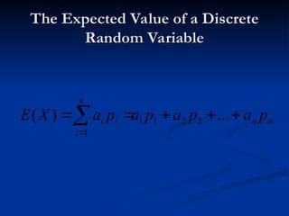
25.
The Expected Valueof a Discrete
The Expected Value of a Discrete
Random Variable
Random Variable
n
n
n
i
i
i p
a
p
a
p
a
p
a
X
E
...
)
( 2
2
1
1
1
26.
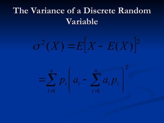
The Variance ofa Discrete Random
The Variance of a Discrete Random
Variable
Variable
2
2
)
(
)
( X
E
X
E
X
n
i
n
i
i
i
i
i p
a
a
p
1
2
1
27.
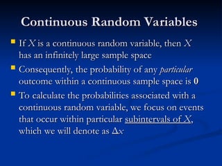
Continuous Random Variables
ContinuousRandom Variables
If
If X
X is a continuous random variable, then
is a continuous random variable, then X
X
has an infinitely large sample space
has an infinitely large sample space
Consequently, the probability of any
Consequently, the probability of any particular
particular
outcome within a continuous sample space is
outcome within a continuous sample space is 0
0
To calculate the probabilities associated with a
To calculate the probabilities associated with a
continuous random variable, we focus on events
continuous random variable, we focus on events
that occur within particular
that occur within particular subintervals of
subintervals of X
X,
,
which we will denote as
which we will denote as Δ
Δx
x
28.
Continuous Random Variables
ContinuousRandom Variables
dx
x
xf
X
E
x
x
f
x
X
E i
n
i
i
)
(
)
(
)
(
)
(
1
x
x
f
x
X
P i
i
)
(
)
(
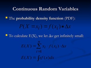
The
The probability density function
probability density function (PDF):
(PDF):
To calculate E(X), we let
To calculate E(X), we let Δ
Δx
x get infinitely small:
get infinitely small:
29.
Uniform Random Variables
UniformRandom Variables
Defined for a
Defined for a closed interval
closed interval (for example,
(for example,
[0,10], which contains all numbers between 0
[0,10], which contains all numbers between 0
and 10,
and 10, including
including the two end points 0 and 10).
the two end points 0 and 10).
0
0.1
0.2
0 1 2 3 4 5 6 7 8 9 10
X
P
(
X
)
Subinterval [5,6]
Subinterval [3,4]
otherwise
x
x
f
,
0
10
0
,
10
/
1
)
(
The probability
density function
(PDF)
30.
Uniform Random Variables
UniformRandom Variables
2
/
)
(
)
( a
b
X
E
For a uniform random variable X, where f(x) is
defined on the interval [a,b] and where a<b:
12
)
(
)
(
2
2 a
b
X
otherwise
b
x
a
a
b
x
f
,
0
),
/(
1
)
(
31.
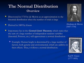
The Normal Distribution
TheNormal Distribution
Overview
Overview
Discovered in 1733 by de Moivre as an approximation to the
Discovered in 1733 by de Moivre as an approximation to the
binomial distribution when the number of trials is large
binomial distribution when the number of trials is large
Derived in 1809 by Gauss
Derived in 1809 by Gauss
Importance lies in the
Importance lies in the Central Limit Theorem
Central Limit Theorem, which states that
, which states that
the sum of a large number of independent random variables
the sum of a large number of independent random variables
(binomial, Poisson, etc.) will approximate a normal distribution
(binomial, Poisson, etc.) will approximate a normal distribution
Example: Human height is determined by a large number of
Example: Human height is determined by a large number of
factors, both genetic and environmental, which are additive in
factors, both genetic and environmental, which are additive in
their effects. Thus, it follows a normal distribution.
their effects. Thus, it follows a normal distribution.
Karl F. Gauss
(1777-1855)
Abraham de Moivre
(1667-1754)
32.
The Normal Distribution
TheNormal Distribution
Overview
Overview
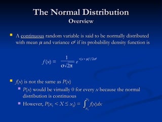
A
A continuous
continuous random variable is said to be normally distributed
random variable is said to be normally distributed
with mean
with mean
and variance
and variance
2
2
if its probability density function is
if its probability density function is
f
f(
(x
x) is not the same as
) is not the same as P
P(
(x
x)
)
P
P(
(x
x) would be virtually 0 for every
) would be virtually 0 for every x
x because the normal
because the normal
distribution is continuous
distribution is continuous
However,
However, P
P(
(x
x1
1 <
< X
X ≤
≤ x
x2
2) =
) = f
f(
(x
x)
)dx
dx
f (x) =
1
2
(x )2
/22
e
x
x1
1
x
x2
2
33.
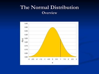
The Normal Distribution
TheNormal Distribution
Overview
Overview
0.00
0.05
0.10
0.15
0.20
0.25
0.30
0.35
0.40
0.45
-3 -2.5 -2 -1.5 -1 -0.5 0 0.5 1 1.5 2 2.5 3
x
f
(
x
)
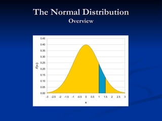
34.
The Normal Distribution
TheNormal Distribution
Overview
Overview
0.00
0.05
0.10
0.15
0.20
0.25
0.30
0.35
0.40
0.45
-3 -2.5 -2 -1.5 -1 -0.5 0 0.5 1 1.5 2 2.5 3
x
f
(
x
)
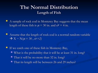
The Normal Distribution
TheNormal Distribution
Length of Fish
Length of Fish
A sample of rock cod in Monterey Bay suggests that the mean
A sample of rock cod in Monterey Bay suggests that the mean
length of these fish is
length of these fish is
= 30 in. and
= 30 in. and
2
2
= 4 in.
= 4 in.
Assume that the length of rock cod is a normal random variable
Assume that the length of rock cod is a normal random variable
X ~ N(
X ~ N(
= 30 ,
= 30 ,
=2)
=2)
If we catch one of these fish in Monterey Bay,
If we catch one of these fish in Monterey Bay,
What is the probability that it will be at least 31 in. long?
What is the probability that it will be at least 31 in. long?
That it will be no more than 32 in. long?
That it will be no more than 32 in. long?
That its length will be between 26 and 29 inches?
That its length will be between 26 and 29 inches?
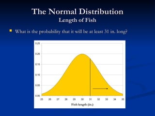
37.
The Normal Distribution
TheNormal Distribution
Length of Fish
Length of Fish
What is the probability that it will be at least 31 in. long?
What is the probability that it will be at least 31 in. long?
0.00
0.05
0.10
0.15
0.20
0.25
25 26 27 28 29 30 31 32 33 34 35
Fish length (in.)
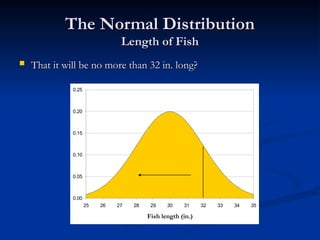
38.
The Normal Distribution
TheNormal Distribution
Length of Fish
Length of Fish
That it will be no more than 32 in. long?
That it will be no more than 32 in. long?
0.00
0.05
0.10
0.15
0.20
0.25
25 26 27 28 29 30 31 32 33 34 35
Fish length (in.)
39.
The Normal Distribution
TheNormal Distribution
Length of Fish
Length of Fish
That its length will be between 26 and 29 inches?
That its length will be between 26 and 29 inches?
0.00
0.05
0.10
0.15
0.20
0.25
25 26 27 28 29 30 31 32 33 34 35
Fish length (in.)
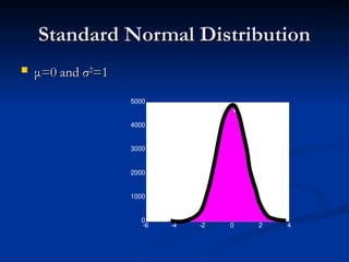
40.
-6 -4 -20 2 4
0
1000
2000
3000
4000
5000
Standard Normal Distribution
Standard Normal Distribution
μ
μ=0 and
=0 and σ
σ2
2
=1
=1
41.
Useful properties ofthe normal
Useful properties of the normal
distribution
distribution
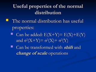
The normal distribution has useful
The normal distribution has useful
properties:
properties:
Can be added: E(X+Y)= E(X)+E(Y)
Can be added: E(X+Y)= E(X)+E(Y)
and
and σ
σ2
2
(X+Y)=
(X+Y)= σ
σ2
2
(X)+
(X)+ σ
σ2
2
(Y)
(Y)
Can be transformed with
Can be transformed with shift
shift and
and
change of scale
change of scale operations
operations
42.
Consider two randomvariables X and Y
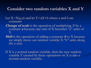
Consider two random variables X and Y
Let X~N(
Let X~N(μ
μ,
,σ
σ) and let Y=aX+b where a and b are
) and let Y=aX+b where a and b are
constants
constants
Change of scale
Change of scale is the operation of multiplying
is the operation of multiplying X
X by a
by a
constant
constant a
a because one unit of X becomes “a” units of
because one unit of X becomes “a” units of
Y.
Y.
Shift
Shift is the operation of adding a constant
is the operation of adding a constant b
b to X because
to X because
we simply move our random variable X “b” units along
we simply move our random variable X “b” units along
the x-axis.
the x-axis.
If X is a normal random variable, then the new random
If X is a normal random variable, then the new random
variable Y created by these operations on X is also a
variable Y created by these operations on X is also a
normal random variable .
normal random variable .
43.
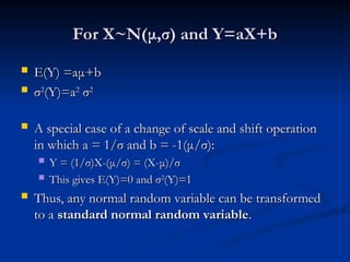
For X~N(
For X~N(μ
μ,
,σ
σ)and Y=aX+b
) and Y=aX+b
E(Y) =a
E(Y) =aμ
μ+b
+b
σ
σ2
2
(Y)=a
(Y)=a2
2
σ
σ2
2
A special case of a change of scale and shift operation
A special case of a change of scale and shift operation
in which a = 1/
in which a = 1/σ
σ and b = -1(
and b = -1(μ
μ/
/σ
σ):
):
Y = (1/
Y = (1/σ
σ)X-(
)X-(μ
μ/
/σ
σ) = (X-
) = (X-μ
μ)/
)/σ
σ
This gives E(Y)=0 and
This gives E(Y)=0 and σ
σ2
2
(Y)=1
(Y)=1
Thus, any normal random variable can be transformed
Thus, any normal random variable can be transformed
to a
to a standard normal random variable
standard normal random variable.
.
44.
The Central LimitTheorem
The Central Limit Theorem
Asserts that standardizing
Asserts that standardizing any
any random variable that itself is a sum
random variable that itself is a sum
or average of a set of independent random variables results in a
or average of a set of independent random variables results in a
new random variable that is “nearly the same as” a standard
new random variable that is “nearly the same as” a standard
normal one.
normal one.
So what? The C.L.T allows us to use statistical tools that require
So what? The C.L.T allows us to use statistical tools that require
our sample observations to be drawn from normal distributions,
our sample observations to be drawn from normal distributions,
even though the underlying data themselves may not be normally
even though the underlying data themselves may not be normally
distributed
distributed!
!
The only caveats are that the sample size must be “large enough”
The only caveats are that the sample size must be “large enough”
and that the observations themselves must be independent and
and that the observations themselves must be independent and
all drawn from a distribution with common expectation and
all drawn from a distribution with common expectation and
variance.
variance.
45.
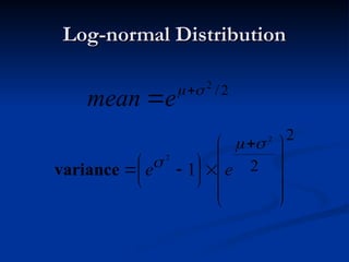
Log-normal Distribution
Log-normal Distribution
X is a
X is a log-normal random
log-normal random
variable
variable if its natural
if its natural
logarithm, ln(X), is a normal
logarithm, ln(X), is a normal
random variable [NOTE:
random variable [NOTE:
ln(X) is same as log
ln(X) is same as loge
e(X)]
(X)]
Original values of X give a
Original values of X give a
right-skewed distribution (A),
right-skewed distribution (A),
but plotting on a logarithmic
but plotting on a logarithmic
scale gives a normal
scale gives a normal
distribution (B).
distribution (B).
Many ecologically important
Many ecologically important
variables are log-normally
variables are log-normally
distributed.
distributed.
rep 1994
1
6
0
0
.
0
1
5
0
0
.
0
1
4
0
0
.
0
1
3
0
0
.
0
1
2
0
0
.
0
1
1
0
0
.
0
1
0
0
0
.
0
9
0
0
.
0
8
0
0
.
0
7
0
0
.
0
6
0
0
.
0
5
0
0
.
0
4
0
0
.
0
3
0
0
.
0
2
0
0
.
0
1
0
0
.
0
0
.
0
300
200
100
0
Std. Dev = 183.79
Mean = 127.5
N = 765.00
SOURCE: Quintana-Ascencio et al. 2006; Hypericum data from Archbold Biological Station
LOGREP94
7
.
2
5
6
.
7
5
6
.
2
5
5
.
7
5
5
.
2
5
4
.
7
5
4
.
2
5
3
.
7
5
3
.
2
5
2
.
7
5
2
.
2
5
1
.
7
5
1
.
2
5
.
7
5
70
60
50
40
30
20
10
0
Std. Dev = 1.44
Mean = 4.00
N = 765.00
A
Exercise
Exercise
Next, wewill perform an exercise in R that will
Next, we will perform an exercise in R that will
allow you to work with some of these
allow you to work with some of these
probability distributions!
probability distributions!
Editor's Notes
#2 P(Capture) = # of captures/# of visits; P(Escape) = # of escapes/# of visits
#3 NOTE: Axiom 1 assumes that the outcomes in the sample space are mutually exclusive and exhaustive.
Use example of randomly shuffled deck of playing cards with 52 cards.

![Uniform Random Variables
Uniform Random Variables
Defined for a
Defined for a closed interval
closed interval (for example,
(for example,
[0,10], which contains all numbers between 0
[0,10], which contains all numbers between 0
and 10,
and 10, including
including the two end points 0 and 10).
the two end points 0 and 10).
0
0.1
0.2
0 1 2 3 4 5 6 7 8 9 10
X
P
(
X
)
Subinterval [5,6]
Subinterval [3,4]
otherwise
x
x
f
,
0
10
0
,
10
/
1
)
(
The probability
density function
(PDF)](https://image.slidesharecdn.com/probabilitydistributions-250418041818-2924d826/85/Probability_Distributions-lessons-with-random-variables-29-320.jpg)
![Uniform Random Variables
Uniform Random Variables
2
/
)
(
)
( a
b
X
E
For a uniform random variable X, where f(x) is
defined on the interval [a,b] and where a<b:
12
)
(
)
(
2
2 a
b
X
otherwise
b
x
a
a
b
x
f
,
0
),
/(
1
)
(](https://image.slidesharecdn.com/probabilitydistributions-250418041818-2924d826/85/Probability_Distributions-lessons-with-random-variables-30-320.jpg)

![Log-normal Distribution
Log-normal Distribution
X is a
X is a log-normal random
log-normal random
variable
variable if its natural
if its natural
logarithm, ln(X), is a normal
logarithm, ln(X), is a normal
random variable [NOTE:
random variable [NOTE:
ln(X) is same as log
ln(X) is same as loge
e(X)]
(X)]
Original values of X give a
Original values of X give a
right-skewed distribution (A),
right-skewed distribution (A),
but plotting on a logarithmic
but plotting on a logarithmic
scale gives a normal
scale gives a normal
distribution (B).
distribution (B).
Many ecologically important
Many ecologically important
variables are log-normally
variables are log-normally
distributed.
distributed.
rep 1994
1
6
0
0
.
0
1
5
0
0
.
0
1
4
0
0
.
0
1
3
0
0
.
0
1
2
0
0
.
0
1
1
0
0
.
0
1
0
0
0
.
0
9
0
0
.
0
8
0
0
.
0
7
0
0
.
0
6
0
0
.
0
5
0
0
.
0
4
0
0
.
0
3
0
0
.
0
2
0
0
.
0
1
0
0
.
0
0
.
0
300
200
100
0
Std. Dev = 183.79
Mean = 127.5
N = 765.00
SOURCE: Quintana-Ascencio et al. 2006; Hypericum data from Archbold Biological Station
LOGREP94
7
.
2
5
6
.
7
5
6
.
2
5
5
.
7
5
5
.
2
5
4
.
7
5
4
.
2
5
3
.
7
5
3
.
2
5
2
.
7
5
2
.
2
5
1
.
7
5
1
.
2
5
.
7
5
70
60
50
40
30
20
10
0
Std. Dev = 1.44
Mean = 4.00
N = 765.00
A](https://image.slidesharecdn.com/probabilitydistributions-250418041818-2924d826/85/Probability_Distributions-lessons-with-random-variables-45-320.jpg)