The document explores composite functions, their applications in real-life scenarios such as the discovery of penicillin, and various probability distributions including binomial, Bernoulli, and Poisson distributions. Each distribution is explained with examples illustrating their significance in fields like education and statistics. Additionally, it discusses continuous probability distributions like normal distribution, including its characteristics and formulas.

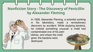
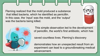
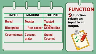
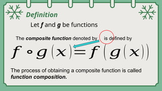
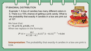
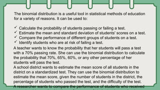
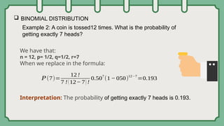
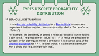
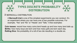
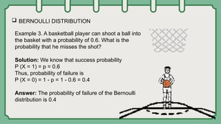
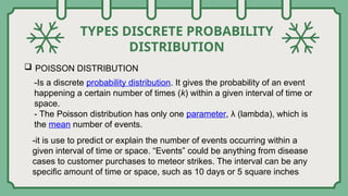
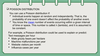
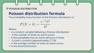
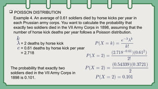
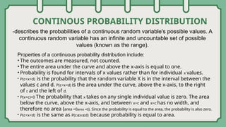
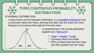
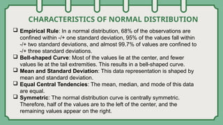
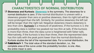
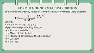
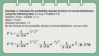
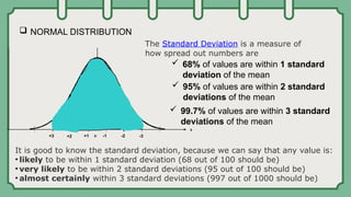
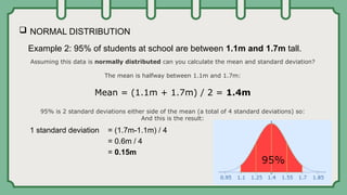
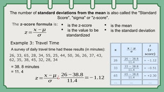
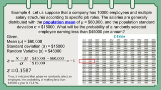
1. COMPOSITE
FUNCTIONS
By:
Ma’am Dolly May S. Palasan

2. PROBABILITY DISTRIBUTION
Recognize the composition of functions
Perform the composition of functions
LEARNING OBJECTIVES
At the end of the lesson, the student shall be
able to :
Appreciate the importance of composite
functions in real-life applications.

3. Nonfiction Story : The Discovery of Penicillin
by Alexander Fleming
In 1928, Alexander Fleming, a scientist working
in his laboratory, made a revolutionary
discovery by accident. While studying bacteria,
he noticed something unusual: a mold had
contaminated one of his petri
dishes, and where the mold
grew, the bacteria were
destroyed.

4. Fleming realized that the mold produced a substance
that killed bacteria, which he identified as penicillin.
In this case, the ‘input’ was the mold, and the ‘output’
was the bacteria being killed.
This simple observation led to the development
of penicillin, the world’s first antibiotic, which has
saved countless lives. Fleming’s discovery
demonstrates how an unexpected result from an
experiment can lead to a groundbreaking medical
advancement.

5. FUNCTION
S
A function
relates an
input to an
output.
INPUT MACHINE OUTPUT
Bread Toaster Toasted
Bread
Rice grains Rice cooker Cooked Rice
Coconut meat Coconut
grater
Grated
Coconut

6. Definition
Let f and g be functions
The composite function denoted by is defined by
𝑓 ∘𝑔 (𝑥 )= 𝑓 ( 𝑔 ( 𝑥))
The process of obtaining a composite function is called
function composition.

7. Example 1.
𝑝( )=
𝑥
𝑔 ∘ 𝑓 ( 𝑥 )= 𝑔 ( 𝑓 ( 𝑥) )
Examples:
For example 1 and 2
Let,
Example 1. Find and simplify
𝑓( )=2 +1
𝑥 𝑥 𝑔( )= ( +1)
𝑥 √ 𝑥
Find and simplify
¿ 𝑔
( 2 𝑥 +1)
¿ √ 𝑥+ 1
+1
¿ √2 𝑥+ 2

8.  BINOMIAL DISTRIBUTION
Example 1: A box of candies has many different colors in
it. There is a 15% chance of getting a pink candy. What is
the probability that exactly 4 candies in a box are pink out
of 10?
We have that:
n = 10, p=0.15, q=0.85, r=4
When we replace in the formula:
Interpretation: The probability that exactly 4 candies in a box are pink is
0.04.
𝑃 (4)=
10 !
4!(10− 4)!
0.15
4
(1−0.15)
10 − 4
=0.04

9. The binomial distribution is a useful tool in statistical methods of education
for a variety of reasons. It can be used to:
 Calculate the probability of students passing or failing a test.
Example.
 Estimate the mean and standard deviation of students' scores on a test.
 Compare the performance of different groups of students on a test.
 Identify students who are at risk of failing a test.
A teacher wants to know the probability that her students will pass a test
with a 70% passing rate. She can use the binomial distribution to calculate
the probability that 70%, 65%, 60%, or any other percentage of her
students will pass the test.
A school district wants to estimate the mean score of all students in the
district on a standardized test. They can use the binomial distribution to
estimate the mean score, given the number of students in the district, the

10. The binomial distribution is a useful tool in statistical methods of education
for a variety of reasons. It can be used to:
 Calculate the probability of students passing or failing a test.
 Estimate the mean and standard deviation of students' scores on a test.
 Compare the performance of different groups of students on a test.
 Identify students who are at risk of failing a test.
A teacher wants to know the probability that her students will pass a test
with a 70% passing rate. She can use the binomial distribution to calculate
the probability that 70%, 65%, 60%, or any other percentage of her
students will pass the test.
A school district wants to estimate the mean score of all students in the
district on a standardized test. They can use the binomial distribution to
estimate the mean score, given the number of students in the district, the
percentage of students who passed the test, and the difficulty of the test.
A researcher wants to compare the performance of students who received

11.  BINOMIAL DISTRIBUTION
Example 2: A coin is tossed12 times. What is the probability of
getting exactly 7 heads?
We have that:
n = 12, p= 1/2, q=1/2, r=7
When we replace in the formula:
Interpretation: The probability of getting exactly 7 heads is 0.193.
𝑃 (7)=
12 !
7 !(12− 7) !
0.50
7
(1− 050)
12−7
=0.193

12. TYPES DISCRETE PROBABILITY
DISTRIBUTION
 BERNOULLI DISTRIBUTION
- is a discrete probability distribution for a Bernoulli trial — a random
experiment that has only two outcomes (usually called a “Success” or a
“Failure”).
For example, the probability of getting a heads (a “success”) while flipping
a coin is 0.5. The probability of “failure” is 1 – P (1 minus the probability of
success, which also equals 0.5 for a coin toss). It is a special case of the
binomial distribution for n = 1. In other words, it is a binomial distribution
with a single trial (e.g. a single coin toss).

13. TYPES DISCRETE PROBABILITY
DISTRIBUTION
 BERNOULLI DISTRIBUTION
A Bernoulli trial is one of the simplest experiments you can conduct. It’s
an experiment where you can have one of two possible outcomes. For
example, “Yes” and “No” or “Heads” and “Tails.” A few examples:
Coin tosses: record how many coins land heads up and how many land tails up.
Births: how many boys are born and how many girls are born each day.
Rolling Dice: the probability of a roll of two die resulting in a double six.

14.  BERNOULLI DISTRIBUTION
Example 3. A basketball player can shoot a ball into
the basket with a probability of 0.6. What is the
probability that he misses the shot?
Solution: We know that success probability
P (X = 1) = p = 0.6
Thus, probability of failure is
P (X = 0) = 1 - p = 1 - 0.6 = 0.4
Answer: The probability of failure of the Bernoulli
distribution is 0.4

15. TYPES DISCRETE PROBABILITY
DISTRIBUTION
 POISSON DISTRIBUTION
-Is a discrete probability distribution. It gives the probability of an event
happening a certain number of times (k) within a given interval of time or
space.
- The Poisson distribution has only one parameter, λ (lambda), which is
the mean number of events.
-it is use to predict or explain the number of events occurring within a
given interval of time or space. “Events” could be anything from disease
cases to customer purchases to meteor strikes. The interval can be any
specific amount of time or space, such as 10 days or 5 square inches.

16.  POISSON DISTRIBUTION
You can use a Poisson distribution if:
 Individual events happen at random and independently. That is, the
probability of one event doesn’t affect the probability of another event.
 You know the mean number of events occurring within a given interval
of time or space. This number is called λ (lambda), and it is assumed to
be constant.
For example, a Poisson distribution could be used to explain or predict:
Text messages per hour
 Male grizzly bears per hectare
 Machine malfunctions per year
 Website visitors per month
 Influenza cases per year

17.  POISSON DISTRIBUTION
Poisson distribution formula
The probability mass function of the Poisson distribution is:
Where:
• is a random variable following a Poisson distribution
• is the number of times an event occurs
• is the probability that an event will occur k times
• is Euler’s constant (approximately 2.718)
• is the average number of times an event occurs
•! is the factorial function

18.  POISSON DISTRIBUTION
Example 4. An average of 0.61 soldiers died by horse kicks per year in
each Prussian army corps. You want to calculate the probability that
exactly two soldiers died in the VII Army Corps in 1898, assuming that the
number of horse kick deaths per year follows a Poisson distribution.
= 2 deaths by horse kick
= 0.61 deaths by horse kick per year
= 2.718
The probability that exactly two
soldiers died in the VII Army Corps in
1898 is 0.101.

19. CONTINOUS PROBABILITY DISTRIBUTION
-describes the probabilities of a continuous random variable's possible values. A
continuous random variable has an infinite and uncountable set of possible
values (known as the range).
Properties of a continuous probability distribution include:
• The outcomes are measured, not counted.
• The entire area under the curve and above the x-axis is equal to one.
• Probability is found for intervals of x values rather than for individual x values.
• P(c<x<d) is the probability that the random variable X is in the interval between the
values c and d. P(c<x<d) is the area under the curve, above the x-axis, to the right
of c and the left of d.
• P(x=c)=0 The probability that x takes on any single individual value is zero. The area
below the curve, above the x-axis, and between x=c and x=c has no width, and
therefore no area (area =0area =0). Since the probability is equal to the area, the probability is also zero.
• P(c<x<d) is the same as P(c≤x≤d) because probability is equal to area.

20. CONTINOUS PROBABILITY DISTRIBUTION
Example 1. Consider the function f(x)120 is a horizontal line. However,
since 0≤x≤20, f(x) is restricted to the portion between x=0 and x=20, inclusive.
f(x)=120 for 0≤x≤20
The graph of f(x)=120 is a horizontal line
segment when 0≤x≤20.
The area between f(x)120.
AREA=20(1/20)=1

21. TYPES CONTINOUS PROBABILITY
DISTRIBUTION
 NORMAL DISTRIBUTION
-is also known as the Gaussian distribution, is a probability distribution that
is symmetric about the mean, showing that data near the mean are more
frequent in occurrence than data far from the mean.
-In graphical form, the normal distribution
appears as a "bell curve".
 mean = median = mode
 symmetry about the center
 50% of values less than the mean
and 50% greater than the mean
Mean
Median
Mode
50% 50%

22. CHARACTERISTICS OF NORMAL DISTRIBUTION
 Empirical Rule: In a normal distribution, 68% of the observations are
confined within -/+ one standard deviation, 95% of the values fall within
-/+ two standard deviations, and almost 99.7% of values are confined to
-/+ three standard deviations.
 Bell-shaped Curve: Most of the values lie at the center, and fewer
values lie at the tail extremities. This results in a bell-shaped curve.
 Mean and Standard Deviation: This data representation is shaped by
mean and standard deviation.
 Equal Central Tendencies: The mean, median, and mode of this data
are equal.
 Symmetric: The normal distribution curve is centrally symmetric.
Therefore, half of the values are to the left of the center, and the
remaining values appear on the right.

23. CHARACTERISTICS OF NORMAL DISTRIBUTION
 Skewness and Kurtosis: Skewness is the symmetry. The skewness for a
normal distribution is zero. If the normal distribution is uneven with a
skewness greater than zero or positive skewness, then its right tail will be
more prolonged than the left. Similarly, for positive skewness the left tail
will be longer than the right tail. Negative skewness means skewness is
less than zero. Kurtosis is a measure of peakiness. If the kurtosis is 3, the
probability data is neither too peaked nor too thin at tails. If the kurtosis
is more than three, then the data curve is heightened with fatter tails.
Alternatively, if the kurtosis is less than three, then the represented data
has thin tails with the peak point lower than the normal distribution.
Kurtosis studies the tail of the represented data. For a normal distribution, the
kurtosis is 3.
 Total Area = 1: The total value of the standard deviation, i.e., the
complete area of the curve under this probability function, is one. Also,
the entire mean is zero.

24. FORMULA OF NORMAL DISTRIBUTION
The Probability Density Function (PDF) of a random variable (X) is given by:
Where;
•- < x < ; - < µ < ; σ > 0
∞ ∞ ∞ ∞
•F(x) = Normal probability Function
•x = Random variable
•µ = Mean of distribution
•σ = Standard deviation of the distribution
•π = 3.14159
•e = 2.71828
𝑭 ( 𝒙 )=
𝟏
𝝈 √𝟐 𝝅
𝒆
−
𝟏
𝟐
(
𝒙 −𝝁
𝝈
)
𝟐

25. Example 4. Calculate the probability density function of normal distribution
using the following data. x = 3, μ = 4 and σ = 2.
Solution: Given, variable, x = 3
Mean = 4 and
Standard deviation = 2
By the formula of the probability density of normal distribution, we can write;
𝑭 ( 𝒙 )=
𝟏
𝝈 √𝟐 𝝅
𝒆
−
𝟏
𝟐
(
𝒙 −𝝁
𝝈
)
𝟐
𝑭 (𝟑)=
𝟏
𝟐√𝟐 𝝅
𝒆
−
𝟏
𝟐
(
𝟑 −𝟒
𝟐
)
𝟐
¿
𝟏
𝟐√𝟐 𝝅
𝒆
−(
𝟑− 𝟒
𝟐
)
𝟐
¿
𝟏
𝟐√𝟐 𝝅
𝒆
−
𝟏
𝟖
¿𝟎.𝟏𝟕𝟔

26.  NORMAL DISTRIBUTION
 68% of values are within 1 standard
deviation of the mean
+1 -1
+2 -2
+3 -3
 95% of values are within 2 standard
deviations of the mean
 99.7% of values are within 3 standard
deviations of the mean
The Standard Deviation is a measure of
how spread out numbers are
It is good to know the standard deviation, because we can say that any value is:
• likely to be within 1 standard deviation (68 out of 100 should be)
• very likely to be within 2 standard deviations (95 out of 100 should be)
• almost certainly within 3 standard deviations (997 out of 1000 should be)

27.  NORMAL DISTRIBUTION
Example 2: 95% of students at school are between 1.1m and 1.7m tall.
1 standard deviation = (1.7m-1.1m) / 4
= 0.6m / 4
= 0.15m
Assuming this data is normally distributed can you calculate the mean and standard deviation?
The mean is halfway between 1.1m and 1.7m:
Mean = (1.1m + 1.7m) / 2 = 1.4m
95% is 2 standard deviations either side of the mean (a total of 4 standard deviations) so:
And this is the result:

28. The number of standard deviations from the mean is also called the "Standard
Score", "sigma" or "z-score".
 is the z-score
 is the value to be
standardized
26, 33, 65, 28, 34, 55, 25, 44, 50, 36, 26, 37, 43,
62, 35, 38, 45, 32, 28, 34
The z-score formula is:
𝑧=
𝑥 −𝜇
𝜎
Example 3: Travel Time
A survey of daily travel time had these results (in minutes):
= 38. 8 minutes
= 11. 4
 is the mean
 is the standard deviation
𝑧=
𝑥 −𝜇
𝜎
¿
26 −38.8
11.4
=−1.12

29. Example 4. Let us suppose that a company has 10000 employees and multiple
salary structures according to specific job roles. The salaries are generally
distributed with the population mean of µ = $60,000, and the population standard
deviation σ = $15000. What will be the probability of a randomly selected
employee earning less than $45000 per annum?
Given,
Mean (µ) = $60,000
Standard deviation (σ) = $15000
Random Variable (x) = $45000
𝑧=
𝑥 −𝜇
𝜎
¿
$45000 −$60,000
$15000
=−1
𝑧=0.1587
Thus, it indicated that when we randomly select an
employee, the probability of making less than
$45000 a year is 15.87%.

30. SAMPLING
DISTRIBUTION

31. SAMPLING DISTRIBUTION