
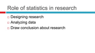
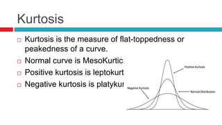
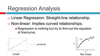
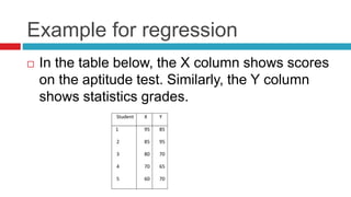
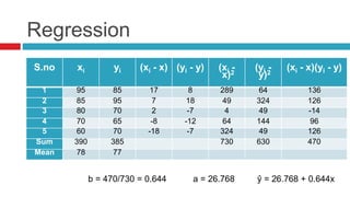
![Linear Regression Equation
Unknown parameter a and b can be calculated by below
formulam = b = slope of line, a= c = intercept
Above formula gives best fit line by using least square method.
b = Σ [ (𝑥𝑖 - 𝑥)(𝑦𝑖 - 𝑦) ] / Σ [ (𝑥𝑖 − 𝑥)2
]
a = 𝑦 - b * 𝑥](https://image.slidesharecdn.com/statisticsinresearch-141010030816-conversion-gate02/85/Statistics-in-research-46-320.jpg)

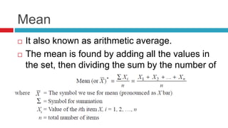
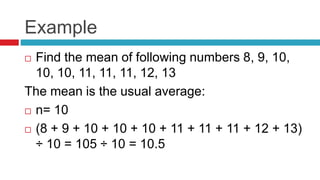
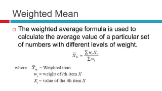
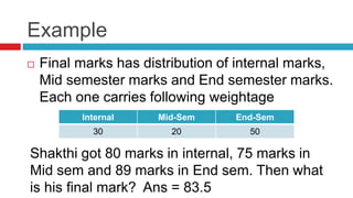
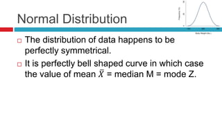
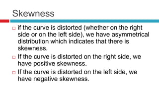
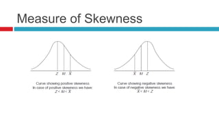
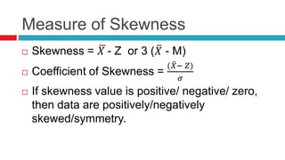
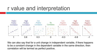
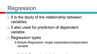
Descriptive statistics are used to summarize and describe characteristics of a data set. It includes measures of central tendency like mean, median, and mode, measures of variability like range and standard deviation, and the distribution of data through histograms. Inferential statistics are used to generalize results from a sample to the population it represents through estimation of population parameters and hypothesis testing. Correlation and regression analysis are used to study relationships between two or more variables.


![Lesson3 lpart one - Measures mean [Autosaved].pptx](https://cdn.slidesharecdn.com/ss_thumbnails/lesson2-measuresmeanautosaved-241011173812-613e1e66-thumbnail.jpg?width=640&height=640&fit=bounds)


![[DSC Europe 25] Gordana Milutinovic Dumbelovic - From Insight to Oversight: A...](https://cdn.slidesharecdn.com/ss_thumbnails/t7dkjsfxqwwzceropjv4-gordana-milutinovicdumbelovic-from-insight-to-oversight-ai-driven-power-bi-moni-260119121559-9e0bf11b-thumbnail.jpg?width=640&height=640&fit=bounds)


![[DSC Europe 25] Laila Kakar - Leveraging AI for Strategic Excellence: Enhanci...](https://cdn.slidesharecdn.com/ss_thumbnails/eykmhrtsqmaaftwkexh7-dsc-lailakakar-1-260119101520-5f3b5616-thumbnail.jpg?width=640&height=640&fit=bounds)
![[DSC Europe 25] Paula Garcia Esteban -Building the Future: The Role of Data S...](https://cdn.slidesharecdn.com/ss_thumbnails/9ld1r1bsqpwve8qfvphy-paula-garcia-esteban-building-the-future-260122103838-4171f5cb-thumbnail.jpg?width=640&height=640&fit=bounds)


![[DSC Europe 25] Marcos Heidemann - Beyond the Hype: Making AI Coding Assistan...](https://cdn.slidesharecdn.com/ss_thumbnails/eexkhvldrjsopspdjbur-marcos-heidemann-beyond-the-hype-getting-real-value-out-of-ai-assisted-coding-260121115910-7e9d41ec-thumbnail.jpg?width=640&height=640&fit=bounds)
![[DSC Europe 25] Tamas Srancsik - How To Teach Your AI Football? An Argument f...](https://cdn.slidesharecdn.com/ss_thumbnails/bcjh1m9xtbosv20ucftb-tamas-srancsik-how-to-teach-your-ai-football-260121115910-08b53e9e-thumbnail.jpg?width=640&height=640&fit=bounds)


![[DSC Europe 25] Milos Belcevic - Product Professional's Journey to Full-Stack...](https://cdn.slidesharecdn.com/ss_thumbnails/1zovd6fgsycdg4wvgvls-milos-belcevic-product-professionals-journey-to-full-stack-product-developer-260123083019-d993120d-thumbnail.jpg?width=640&height=640&fit=bounds)
![[DSC Europe 25] Jovan Sumarac - Real-World Applications of Computer Vision in...](https://cdn.slidesharecdn.com/ss_thumbnails/fiksms22smcpopvvld03-jovan-sumarac-real-life-applications-of-computer-vision-in-automotive-systems-260120105855-de622abb-thumbnail.jpg?width=640&height=640&fit=bounds)
