Excel 2007
Using Conditional Formatting
Introduction
Conditional Formatting
Watch the video! (5:17min) - Tips for watching our videos.
Download the example to work along with the video.
The Conditional Formatting Options
You have many conditional formatting rules, or options, that you can apply to cells in your spreadsheet. Each
rule will affect selected cells differently. Before you choose a formatting rule, you need to identify what questions
you are trying to answer. For example, in a sales spreadsheet, you might want to identify the salespeople with
lower than average sales. To do this, you need to choose a conditional formatting rule that will show you this
answer. Not all of the options will provide you with this information.
Some of the Conditional Formatting Options Include:
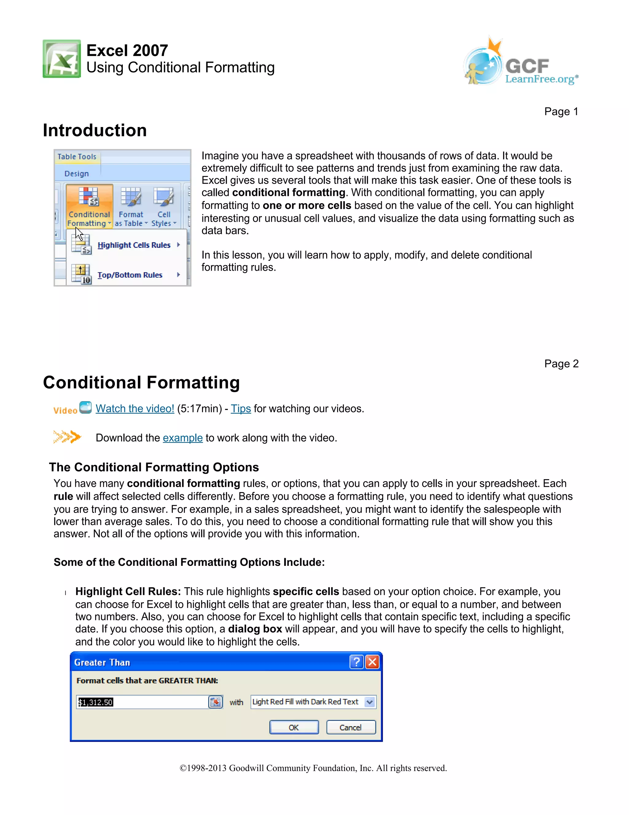
Š Highlight Cell Rules: This rule highlights specific cells based on your option choice. For example, you
can choose for Excel to highlight cells that are greater than, less than, or equal to a number, and between
two numbers. Also, you can choose for Excel to highlight cells that contain specific text, including a specific
date. If you choose this option, a dialog box will appear, and you will have to specify the cells to highlight,
and the color you would like to highlight the cells.
Page 1
Imagine you have a spreadsheet with thousands of rows of data. It would be
extremely difficult to see patterns and trends just from examining the raw data.
Excel gives us several tools that will make this task easier. One of these tools is
called conditional formatting. With conditional formatting, you can apply
formatting to one or more cells based on the value of the cell. You can highlight
interesting or unusual cell values, and visualize the data using formatting such as
data bars.
In this lesson, you will learn how to apply, modify, and delete conditional
formatting rules.
Page 2
©1998-2013 Goodwill Community Foundation, Inc. All rights reserved.
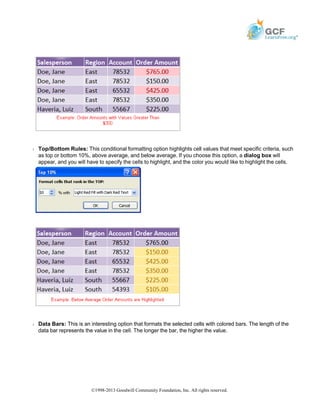
Š Top/Bottom Rules: This conditional formatting option highlights cell values that meet specific criteria, such
as top or bottom 10%, above average, and below average. If you choose this option, a dialog box will
appear, and you will have to specify the cells to highlight, and the color you would like to highlight the cells.
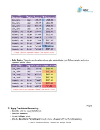
Š Data Bars: This is an interesting option that formats the selected cells with colored bars. The length of the
data bar represents the value in the cell. The longer the bar, the higher the value.
©1998-2013 Goodwill Community Foundation, Inc. All rights reserved.
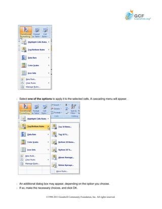
Š Color Scales: This option applies a two or three color gradient to the cells. Different shades and colors
represent specific values.
To Apply Conditional Formatting:
Š Select the cells you would like to format.
Š Select the Home tab.
Š Locate the Styles group.
Š Click the Conditional Formatting command. A menu will appear with your formatting options.
Page 3
©1998-2013 Goodwill Community Foundation, Inc. All rights reserved.
Š Select one of the options to apply it to the selected cells. A cascading menu will appear.
Š An additional dialog box may appear, depending on the option you choose.
Š If so, make the necessary choices, and click OK.
©1998-2013 Goodwill Community Foundation, Inc. All rights reserved.
To Remove Conditional Formatting Rules:
Š Click the Conditional Formatting command.
Š Select Clear Rules. A cascading menu appears.
Š Choose to clear rules from the entire worksheet or the selected cells.
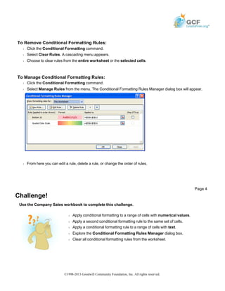
To Manage Conditional Formatting Rules:
Š Click the Conditional Formatting command.
Š Select Manage Rules from the menu. The Conditional Formatting Rules Manager dialog box will appear.
Š From here you can edit a rule, delete a rule, or change the order of rules.
Challenge!
Use the Company Sales workbook to complete this challenge.
Page 4
Š Apply conditional formatting to a range of cells with numerical values.
Š Apply a second conditional formatting rule to the same set of cells.
Š Apply a conditional formatting rule to a range of cells with text.
Š Explore the Conditional Formatting Rules Manager dialog box.
Š Clear all conditional formatting rules from the worksheet.
©1998-2013 Goodwill Community Foundation, Inc. All rights reserved.

Print17

  • 1.
    Excel 2007 Using ConditionalFormatting Introduction Conditional Formatting Watch the video! (5:17min) - Tips for watching our videos. Download the example to work along with the video. The Conditional Formatting Options You have many conditional formatting rules, or options, that you can apply to cells in your spreadsheet. Each rule will affect selected cells differently. Before you choose a formatting rule, you need to identify what questions you are trying to answer. For example, in a sales spreadsheet, you might want to identify the salespeople with lower than average sales. To do this, you need to choose a conditional formatting rule that will show you this answer. Not all of the options will provide you with this information. Some of the Conditional Formatting Options Include: Š Highlight Cell Rules: This rule highlights specific cells based on your option choice. For example, you can choose for Excel to highlight cells that are greater than, less than, or equal to a number, and between two numbers. Also, you can choose for Excel to highlight cells that contain specific text, including a specific date. If you choose this option, a dialog box will appear, and you will have to specify the cells to highlight, and the color you would like to highlight the cells. Page 1 Imagine you have a spreadsheet with thousands of rows of data. It would be extremely difficult to see patterns and trends just from examining the raw data. Excel gives us several tools that will make this task easier. One of these tools is called conditional formatting. With conditional formatting, you can apply formatting to one or more cells based on the value of the cell. You can highlight interesting or unusual cell values, and visualize the data using formatting such as data bars. In this lesson, you will learn how to apply, modify, and delete conditional formatting rules. Page 2 ©1998-2013 Goodwill Community Foundation, Inc. All rights reserved.
  • 2.
    Š Top/Bottom Rules:This conditional formatting option highlights cell values that meet specific criteria, such as top or bottom 10%, above average, and below average. If you choose this option, a dialog box will appear, and you will have to specify the cells to highlight, and the color you would like to highlight the cells. Š Data Bars: This is an interesting option that formats the selected cells with colored bars. The length of the data bar represents the value in the cell. The longer the bar, the higher the value. ©1998-2013 Goodwill Community Foundation, Inc. All rights reserved.
  • 3.
    Š Color Scales:This option applies a two or three color gradient to the cells. Different shades and colors represent specific values. To Apply Conditional Formatting: Š Select the cells you would like to format. Š Select the Home tab. Š Locate the Styles group. Š Click the Conditional Formatting command. A menu will appear with your formatting options. Page 3 ©1998-2013 Goodwill Community Foundation, Inc. All rights reserved.
  • 4.
    Š Select oneof the options to apply it to the selected cells. A cascading menu will appear. Š An additional dialog box may appear, depending on the option you choose. Š If so, make the necessary choices, and click OK. ©1998-2013 Goodwill Community Foundation, Inc. All rights reserved.
  • 5.
    To Remove ConditionalFormatting Rules: Š Click the Conditional Formatting command. Š Select Clear Rules. A cascading menu appears. Š Choose to clear rules from the entire worksheet or the selected cells. To Manage Conditional Formatting Rules: Š Click the Conditional Formatting command. Š Select Manage Rules from the menu. The Conditional Formatting Rules Manager dialog box will appear. Š From here you can edit a rule, delete a rule, or change the order of rules. Challenge! Use the Company Sales workbook to complete this challenge. Page 4 Š Apply conditional formatting to a range of cells with numerical values. Š Apply a second conditional formatting rule to the same set of cells. Š Apply a conditional formatting rule to a range of cells with text. Š Explore the Conditional Formatting Rules Manager dialog box. Š Clear all conditional formatting rules from the worksheet. ©1998-2013 Goodwill Community Foundation, Inc. All rights reserved.