The pivot tables are not created mechanically. In Microsoft excel the user should select the data first for which the pivot table should be created. The pivot table option is available on the insert tab. The user has the option of inserting the pivot table either in the existing sheet or creating the pivot table in the new sheet. Copy the link given below and paste it in new browser window to get more information on Pivot Table:- http://www.transtutors.com/homework-help/statistics/pivot-table.aspx
Presentation is about advance excel advance feature PIVOT Table and contains steps to insert pivot table and some useful features of pivot table in case of large amount of data
Microsoft Excel is one of the greatest, most powerful, most important software applications of all time. Many in the industry will no doubt object. But it provides enormous capacity to do quantitative analysis, letting you do anything from statistical analyses of databases with hundreds of thousands of records to complex estimation tools with user-friendly front ends. And unlike traditional statistical programs, it provides an intuitive interface that lets you see what happens to the data as you manipulate them.
The difference between Tableau’s Groups and Tableau Sets was something that confused me a little when first started with Tableau. Tableau groups seem pretty self-explanatory, but sets seemed a little complicated.
Steps to solve Transportation models by North west corner method are given the presentation. North west corner method is one of the well known methods used to solve the transportation models.
MS Excel Learning for PPC Google AdWords Training CourseRanjan Jena
MS Excel learning to get expertise in Google AdWords training course. Learn all important tips and techniques in MS Excel for your fast and easy approach to Google AdWords analysis and reporting formats.
Ranjan Jena conducts Adwords Training session in Bangalore, currently with more than 45 students already graduated under his guidance and mentorship. For any training need, you can directly reach him at +91-7760969452
The Power of Business Model Pivots: How Underdogs Slay Top Dogs in Business a...Rod King, Ph.D.
What do startups like Twitter, GroupOn, and PayPal have in common? Each of these startups changed a vital block of their initial business model; in other words, they pivoted to a more successful business model and strategy. In contrast, companies such as Kodak and Blockbuster went bankrupt because they failed to pivot on their strategy and business model.
This presentation offers a visual framework - Business Model Pivot (BMP)-Mind Map - for summarizing and discussing business model pivots as well as generating ideas for business model innovation and disruption.
Ias sl atrack-guard tour monitoring ver1indusaviation
SLA-Track a Guard tour Monitoring System developed by Indus Aviation Systems , SLA-Track will help you to secure your Property area and valuable assets . Guard tour monitoring systems ensures proof of presence while Patrolling.
The role of Risk Assessment and Risk Management is to continuously Identify, Analyze, Plan, Track, Control, and Communicate the risks associated with a project.
The Webster’s definition of risk is the possibility of suffering a loss. Risk in itself is not bad. Risk is essential to progress and failure is often a key part of learning. Managing risk is a key part of success.
This document describes the foundations for conducting a risk assessment of a large-scale system development project. Such a project will likely include the procurement of Commercial Off The Shelf (COTS) products as well as their integration with legacy systems.
Example of the stage-gate product management process (sometimes referred to as the phase-gate process). This type of process is used to bring new products or updates to market. At the completion of each phase, there is general a review of the project along with a go / no go / hold / rework decision.
The processes are separated into colors according to knowledge areas and process groups. Based on The Standard for Program Management — Third Edition. Developed under permission from Project Management Institute.
From this power point you can get the details about Advanced Filter, Use of Macros with Advanced Filter, Data Validation, Creation of data validation Drop-Down List, Handling of External Data, Goal Seek, What-if analysis,
MANAGEMENT OF DATABASE INFORMATION SYSTEM
Quering database
Queries are the fastest way to search for information in a database. A query is a database feature that enables the user to display records as well to perform calculations on fields from one or multiple tables.
You can analyze a table or tables by using:-
1. Select query or
2. An action query
Action query:-These are queries that are used to make changes in many records at once. They are mostly used to delete, update, add a group of records from one table to another, or create a new table from another table.
Types of action query in Microsoft Access are:-
1. Update-update data in a table.
2. Append query-add data in a table from one or more tables.
3. Make table Query-Creates a new table from a dynaset
4. Delete query-Delete specified records from one or more tables.
Select query
Is a type of query used for searching and analyzing data in one or more tables. It lets the user specify the search criteria and the records that meet those criteria displayed in a dynaset or analyzed depending on the user requirement.
Creating a selected query
1. Ensure that the database you want to create a query for is open
2. Click the query tab, then new
3. In the new query dialog box, choose either to create a query from in Designing view or using Wizard
4. To design from scratch, click design view. The show table dialo
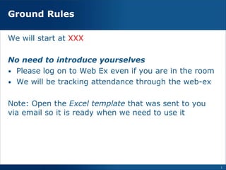
1. Ground Rules
We will start at XXX
No need to introduce yourselves
• Please log on to Web Ex even if you are in the room
• We will be tracking attendance through the web-ex
Note: Open the Excel template that was sent to you
via email so it is ready when we need to use it
1
2. MS Excel 201
Training:
– Conditional
Formatting
– Data Validation
– Pivots and
– Slicers
JH PMO
Speaker: JB Braly
4. Intro to Concepts
Conditional Formatting and Data Validation
Conditional Formatting
•Automatic formatting that is triggered by
conditions that you define.
•Use: Great way to visually highlight
important information in a worksheet.
•Ex: Use to automatically change the color
of cells that contain values greater than or
less certain values, or create a bar graph
based on % complete
Data Validation
•Allows you to restrict the data entered
into a range of cells in an Excel worksheet.
•Use: If you have a worksheet that others
use, ensure only data that matches your
requirements is entered into those cells
•Ex: a range of numbers (e.g. between 10
and 20), only specific text (e.g., High,
Med, Low)
4
5. Intro to Concepts
Pivot Tables and Slicers
Pivot Tables
•Automatically groups, sorts, counts,
totals or averages data stored in table,
displaying the results in a second table
[Pivot] showing the summarized data.
•Use: change the summary's structure by
dragging and dropping fields graphically.
Slicers
•Extension of a pivot table which makes the
job of filtering the pivot table data easier.
•Use: Instead of using the filter drop downs,
use slicers. They act like buttons, that give
you visual reference of what the pivot table
is filtered on.
•Note: You will see why Data Validation is
important when using slicers
5
7. Conditional Formatting
Intro
With conditional formatting, you can select one or more cells,
and create rules (conditions):
• When [i.e. When the cell is High Risk]
• How those cells are formatted [i.e. than make those cells Red]
If the rules (conditions) that you specified are met, then the
formatting is applied.
• The conditions can be, based on the selected cell's contents, or
based on the contents of another cell.
7
Note: You can only control the following formats:
• Font: type, style, and color (but not font size)
• Fill: color and pattern
• Border: color and border (but not border thickness)
• Number (#) format
9. Conditional Formatting
Example 1 – Data Bars
3. Select Data Bars and
Select Blue solid fill
9
You can make a # or % automatically create a visual bar Chart.
Helpful when tracking tasks to show visually how complete they are
* Open First tab of Excel Worksheet
1. Select Cells
to format
2. Select Home tab and Select
Conditional Formatting
Perform
this Step
11. Conditional Formatting
Other cool formats that look hard but are easy
1. Select Highlight
Cells Rules
2. Select Greater
than or Less
than to highlight
cells that are
higher or lower
than those values
11
Highlight CellsTop Bottom Rules
1. Select Top/Bottom Rules
2. Select Above or Below
Average to highlight cells that
are performing above or below
average
Keep Cells Highlighted, then Click Home tab
Perform
this Step
12. Conditional Formatting
Other cool formats that look hard but are easy
12
Color Scales
Select Color Scales to give
you a heat map of the numbers
Icon Sets
Select Icon Sets to
display objects like
Arrows, stop lights, and
pie charts
Click Home tab, then Conditional Formatting:
Perform
this Step
13. Conditional Formatting
How to change the formatting once created
1. Select the cells that are
formatted then click Conditional
Formatting
2. Select Manage Rules
13
4. Here you can change:
• Format Style [i.e. Which Icon]
• Which values give you
• Which color or style
Here you can change:
• Which cells formats apply to
• Which formats that are used
3. Double Click the rule listed
below to edit it.
Tip: You
can select
this if you
want to
hide
numbers
and only
show icon
Perform
this Step
16. Conditional Formatting
Example 2 – Compare Two Columns
When trying to compare two columns, like Baseline vs Actual
16
1. Select cell [F2] you want to format
2. Select New Rule
4. Actual Cell will show the following
3. Click and format highlighted fields.
=E2
** Hit F4 to remove $ before and after E
Perform
this Step
* Open Next tab
18. Conditional Formatting
Example 2 – Compare (cont)
To apply formatting to the other cells below
1. Click on the cell you formatted
2. Hover over the bottom right corner; see plus sign
3. Click your mouse and drag highlighted cell down
18
5. It should look like
this.
To ensure that the cells retained their Original Value
4. Click on this and select Fill Formatting Only
6. To make other cells
Green:
• Add a new rule,
• Use less than in
Drop Down
• Select Format,
• Select Fill tab, then
select green.
Perform
this Step
20. Conditional Formatting
Cond. Formatting - Completed Tab
20
Your final versions of the 2 worksheets should look like this
** Note: If they don’t, go to
Manage Rules on this tab to see
how it was created and find your
error.
22. Data Validation
Intro
In Project Mgt, you often want to have a controlled list [drop
downs] for fields that have a limited number of responses.
22
PMF phases:
5 phases. Ever wish you didn’t have to type it out each
time since it will always only be one of the 5?
Owner:
For action registers – you
always have the same core
group of people that will be
assigned action. Why type
their name each time?
Status:
How many status’ can there be? Not
many
[Not started, In Progress, Complete]
Health:
How many health’s can
there be? [Green,
Yellow, Red]
Risk:
[High, Med, Low]
23. Data Validation
Blank Tab
Below the chart, you will see “Lookups” – which we will use to
build data validation lists
23
Each Column’s validation lists or “Look ups” are directly below each
corresponding Column
Go to next Tab:
24. Data Validation
Select Data that will Receive Drop Downs
1. Select Column of PMF Phases I4:I13 cells to apply validation
lists to
24
2. Select Data on the Menu Bar, then Click Data Validation,
and Select Data Validation again in drop down
Perform
this Step
25. Data Validation
Select Drop Down Info
25
3. Under Settings, and Allow,
select List in drop down
Perform
this Step
4. Under Source, select the graph
with the arrow
5. Select the cells in the Lookups
for the PMF Phases
6. Hit Enter on your keyboard.
7. Click Ok
27. Data Validation
Make More Drop Downs
27
You should now see an arrow to the
right of all the cells selected under
PMF Phases
Perform
this Step
When you select the arrow, there is now a
“validation list” that shows those values
Now Repeat these same steps for
the remaining columns.
28. Data Validation - Tips and tricks
List Source – Direct Input
28
Tip: You can type the lookups or lists directly into the source,
which is helpful when you want to hide the lookups
29. Data Validation
View Formatting Already Applied
29
* Open the Data Validation – Completed Tab
Notice that the Overall Health and Risk Rating have
Conditional Formatting applied.
To view or change the formatting,
1. Select the cells that are formatted,
2. Select Conditional Formatting on the menu ribbon,
3. Select Manage Rules: apply the conditional formats
Perform
this Step
31. Pivots - Intro
Why organize data into Pivot Table?
When you have a lot of data, it can sometimes be difficult to
analyze all of the information in your worksheet.
Why organize list data into a Pivot Table?
• Performs calculations from a spreadsheet WITHOUT having to
input any formulas or copy any cells.
• Helps make worksheets more manageable by summarizing
data and allowing you to manipulate it in different ways.
• To find relationships or gaps within the data that are
otherwise hard to see because of the amount of detail
• To organize the data into a format that’s easy to graph or
chart
31
32. Pivots - Intro
What’s required to make a Pivot Table?
Data used to create a Pivot Table must be in Excel list format:
• All the data in a column is the same kind of data,
• Headers are at the top of each column,
• All the data is located in one place with no gaps.
Ensure that your data meets pivot table needs. Basic criteria:
• Include at least 1 column with duplicate values.
• It should include numerical information.
32
33. Pivots
Start on the Data Validation – Completed Tab
To create a Pivot table, highlight all of the fields below
33
1. Go to the Insert
Tab, then select
Pivot table
2. Select Existing Worksheet,
then select A1
Perform
this Step
36. Pivots
Build Pivot Table
• Drag each of the Pivot Table Fields into the
corresponding Rows and Values
36
Perform
this Step
37. Pivots
Change Date from Count to Sum
In the “Field List” of the Pivot table [on
the bottom right]
37
Perform
this Step
1. Select the Drop down arrow in the Values section
where it says “Count Of Due Date”
2. Select Value Field Settings
3. Select Sum, then click OK
38. Pivots
Fix the format so it looks like a Date
In same Value Field Settings Screen
1. Select Number Format
38
Perform
this Step
2. On Number tab, select Date
3. In the Type section: select
14-Mar-12
4. Click Ok
40. Pivots
Add remaining values to the fields
You should now have the Sum for Due dates.
*Time to add the remaining values:
1. Drag % Complete, Baseline and Actual to values field
It should look like this when you are done.
Perform
this Step
2. Click on Arrow on right of % Complete
3. Go to Value Field Settings, and Change to Average
4. Click on Arrow on right of Baseline and Actual
5. Change to Sum
42. Pivots
Show in a Table
Still looks weird?
42
1. Make the columns look more like a
spreadsheet, left to right:
Another Way:
• Right Click,
Select Pivot
Table Options
• Select Display
tab
• Check Classic
Pivot Table
Perform
this Step
To make yours look like this:
43. Pivots
Remove Subtotals
2. Remove all Subtotals
43
Another way:
• Go to each column
• Right click
• Deselect Subtotal
“XXX”
Perform
this Step
44. Pivots
Adding Conditional Formatting
1. Highlight cells in Overall Health Column
2. Go to Home ribbon and select Format Painter
44
Perform
this Step
To Apply the same conditional formatting from previous tab
• Go to Data Validation – Completed tab
4. Highlight all of the cells in the overall health
column that you want that format to apply to
3. Select the Pivot tab
5. Repeat for Risk Rating
6. Repeat for Actual
46. Pivots – Lets Play
Re-Ordering Columns & Rows
46
Move Columns & Rows around :
Note: if you move column that has conditional formatting applied, formatting
will be lost.
• Click on column header
(drag column left or
right)
• or Row category (drag
up or down).
1. Right Click on a column or row
2. Select Move.
3. Select Move to [any direction]
Another way to do this:
Perform
this Step
47. Pivots – Tips and Tricks
Change Source Data
Sometimes, you add columns or rows below or to the right of the initial
data and need to update Pivot to reflect this addition
1. Click inside any cell in the pivot table, go to the Analyze tab,
2. Select Change Source data, then select it again in the drop down
47
3. Highlight revised Range including column headers, then click enter,
then click Ok
*Now your Pivot table will update and
include new data
Perform
this Step
48. Pivots – Tips and Tricks
Refresh Data in Pivot with Updates
If you made updates inside the original range without changing the
source data, and want your updates to be reflected in the Pivot:
48
*Now your Pivot table will include any new
data
Perform
this Step
One time:
1. Click inside any cell in the pivot table, go to
the Analyze tab
2. Select Refresh, then select Refresh All in
the drop down
Every time you open file:
1. Click inside any cell in the pivot table
2. Right Click
3. Select PivotTable Options
4. Select Data Tab
5. Check Refresh Data When Opening File
6. Retain Items: Change Automatic to None
*Now your Pivot table will update automatically when you just open the file [from closed]
49. Pivots – Tips and Tricks
Prevent Stuff from Moving
Does it bother you when all your columns and Rows move automatically
based on size of the data selected?
49
Perform
this Step
1. Click inside any cell in the pivot
table
2. Right Click
3. Select PivotTable Options
4. Select Layout and Format Tab
5. UnCheck Autofit Widths on
Update
*Now it won’t move
51. Slicers
Intro
• Have you ever wanted to look at data a few different ways?
• Ever wished that you didn’t have to make 5 spreadsheets
to view it in those different “views” per BU or customer?
• You only want to look at open actions
• You only want to look at high risk
• You only want to look at something in a particular
phase
• Or – maybe you wanted to look at things that have
two conditions: Low risk in Deliver Phase.
• Now you can --- Slicers are the answer.
51
52. Slicers
Insert Slicer
After creating a Pivot table, there are only 2 main steps:
1. Click any where in the pivot table
2. Click on the Insert Ribbon, and select Slicer
52
Perform
this Step
Everything that has a name in the columns will have
the option of having a slicer.
3. Check ALL of the but Due date and Deliverable
Go to Slicers Tab to begin
53. Slicers
Slicers Displayed
You will now see the slicers for
all of those displayed like this
• Notice that all values in each
column are now “Buttons”
• Data Validation lists limit the
number of variations you
will see on these slicers
53
Do you see why we created
Data Validation Lists?
55. Slicers
Reposition Slicer Boxes
Now its just up to us to put these slicers in a way
location that is pretty and user friendly
Start by dragging each of the Slicers above the
respective column
• Why are yours different color?
• Why are your buttons smaller?
55
Perform
this Step
56. Slicers – Tips and Tricks
Change Colors
To make the slicers different colors,
• Select the slicer that you want to color
• Go to the Options tab,
• Select the Format or Color
56
Perform
this Step
57. Slicers – Tips and Tricks
Change Height
To make the buttons smaller:
• Click on the slicer(s)
• Right click and select “size and
properties”
57
Perform
this Step
To Decrease the Button Height
Go to Position and Layout, and
then under Button Height,
decrease it to .2” by using the
down arrow once
To prevent slicers from moving:
to prevent your slicers from
moving when columns shrink
or expand, go to Properties,
and then don’t move or size
with cells
59. Slicers – Lets Play
Clear and Select only a few Filters
Lets Play:
1. Click on multiple slicers’
buttons
– See how the pivot below changes base
on those filters
59
Note: To only select a few filters, click on one of the buttons on a slicer,
then hold down CTRL until you are finished selecting all that you want
Perform
this Step
2. Clear slicers by clicking on the X
Notice how some filters get greyed out? This
is because they don’t apply based on the
filters selected
60. Slicers - Tips and Tricks
Link Slicers from 2 Pivots
If you have more than one pivot table using the same source data, you
can Link the slicers:
60
1. Click anywhere in pivot table
2. Go to Analyze Tab
3. Select Filter Connections
Here you can check and
uncheck which
connections the slicers
are linked to from this
and other worksheets
that use the same
source data
Note that when you uncheck it – it no longer updates that Pivot table
Perform
this Step
61. Slicers - Tips and Tricks
Change Slicer Name
61
If you want to change the Name of the slicer without changing the name
of the column from the original Source data:
If you Select Slicer Settings, you
can also change it on this
Perform
this Step
1. Click on one of the slicers
2. Go to Options Tab
You can change the name right
above Slicer Settings
65. Helpful References
Conditional Formatting
• 10 Cool Ways to Use Excels Conditional Formatting
• Easy Excel Examples for Conditional Formatting
Data Validation
• How to Use other Features in Data Validation
Pivots
• Pivot Tables in Excel - EASY Excel Tutorial
• How to Create a Pivot Table in Excel
• Pivot Tables - Five Minute Lessons
• How to Group Months
• Connect Slicers to Multiple Excel Pivot Tables
Slicers
• Use slicers to filter PivotTable data
Charts
• Tips for Pivot Charts
65