Download 11-incredible-excel-conditional-formatting-tricks

Excel Tip | Excel Forum
11 Incredible Excel Conditional Formatting
ADVANCE WAYS OF CONDITIONAL FORMATTING
[www.exceltip.com | www.exceforum.com]
Copyright © 2003 ExcelTip.com, Excelforum.com registered trademark of Microsoft Corporation

www.exceltip.com / www.excelforum.com 11 Incredible Excel Conditional Formatting Tricks 1
© 2015 excelforum.com & exceltip.com
Self-Publishing
ALL RIGHTS RESERVED. This book contains material protected under International and
Federal Copyright Laws and Treaties. Any unauthorized reprint or use of this material is
prohibited. No part of this book may be reproduced or transmitted in and form or by any
means, electronic or mechanical, including photocopying, recording, or by any information
storage and retrieval system without express written permission from the author /
publisher.
The information in this book is provided on as-is basis. The authors and publisher shall have
neither liability nor responsibility to any person or entity with respect to any loss or
damages arising from the information contained in this book.
Author- Excel Forum.com and Exceltip.com
Cover Design-excelforum.com
Published by- Self-publishing
First Published in- June-2015

Microsoft Excel is having so many
unbelievable capabilities that are not instantly perceived. In which Conditional Formatting is
one of the option.
Conditional Formatting is the tool that used to format the cell or a range in the specific
condition. We can use this option on the value of the cell or value of formula, it means if
you have formula in cell then we can specify the value in “Conditional Formatting” of if we
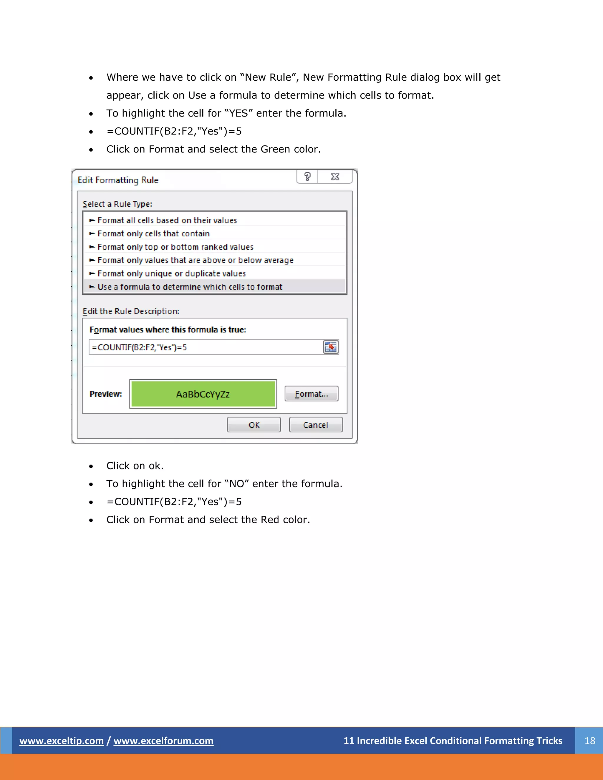
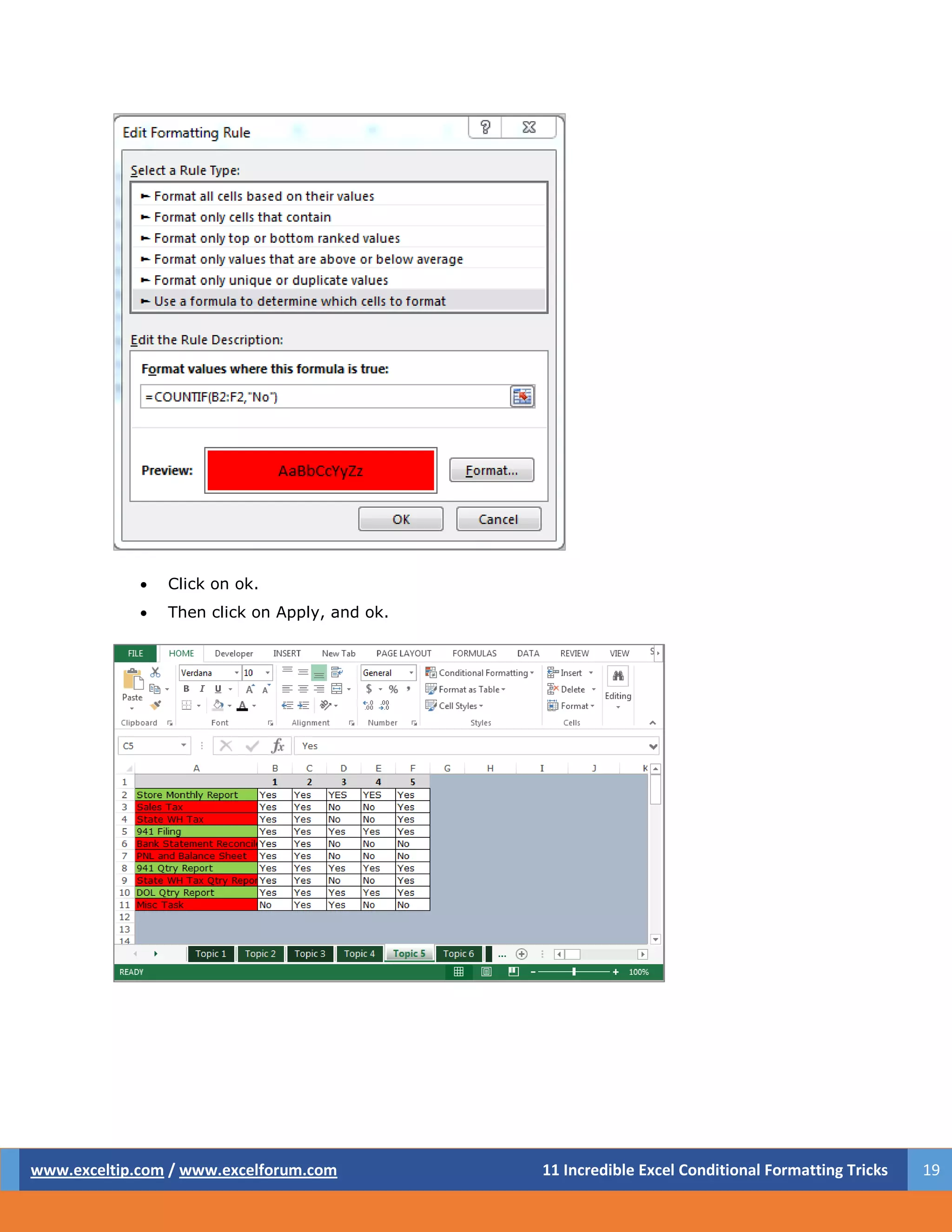
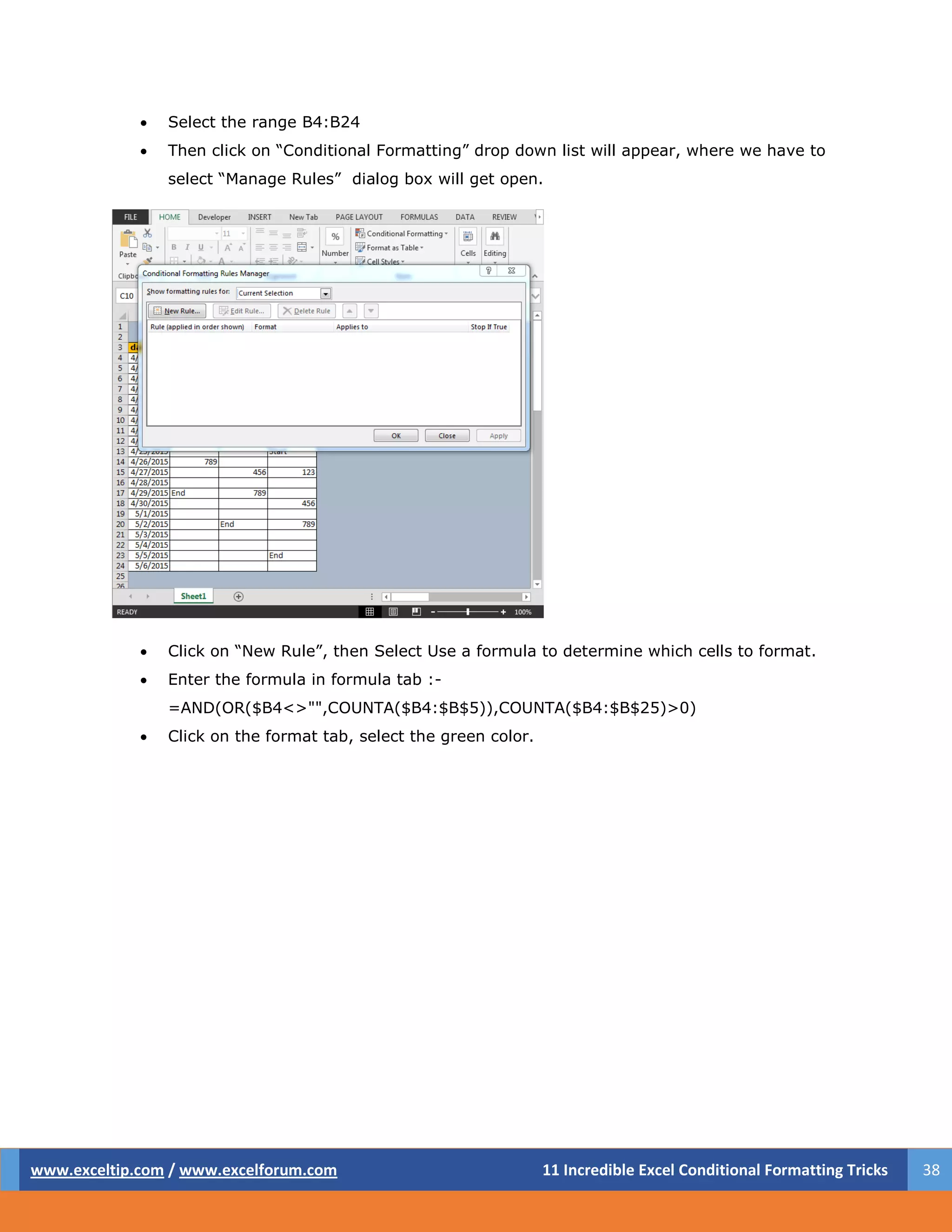
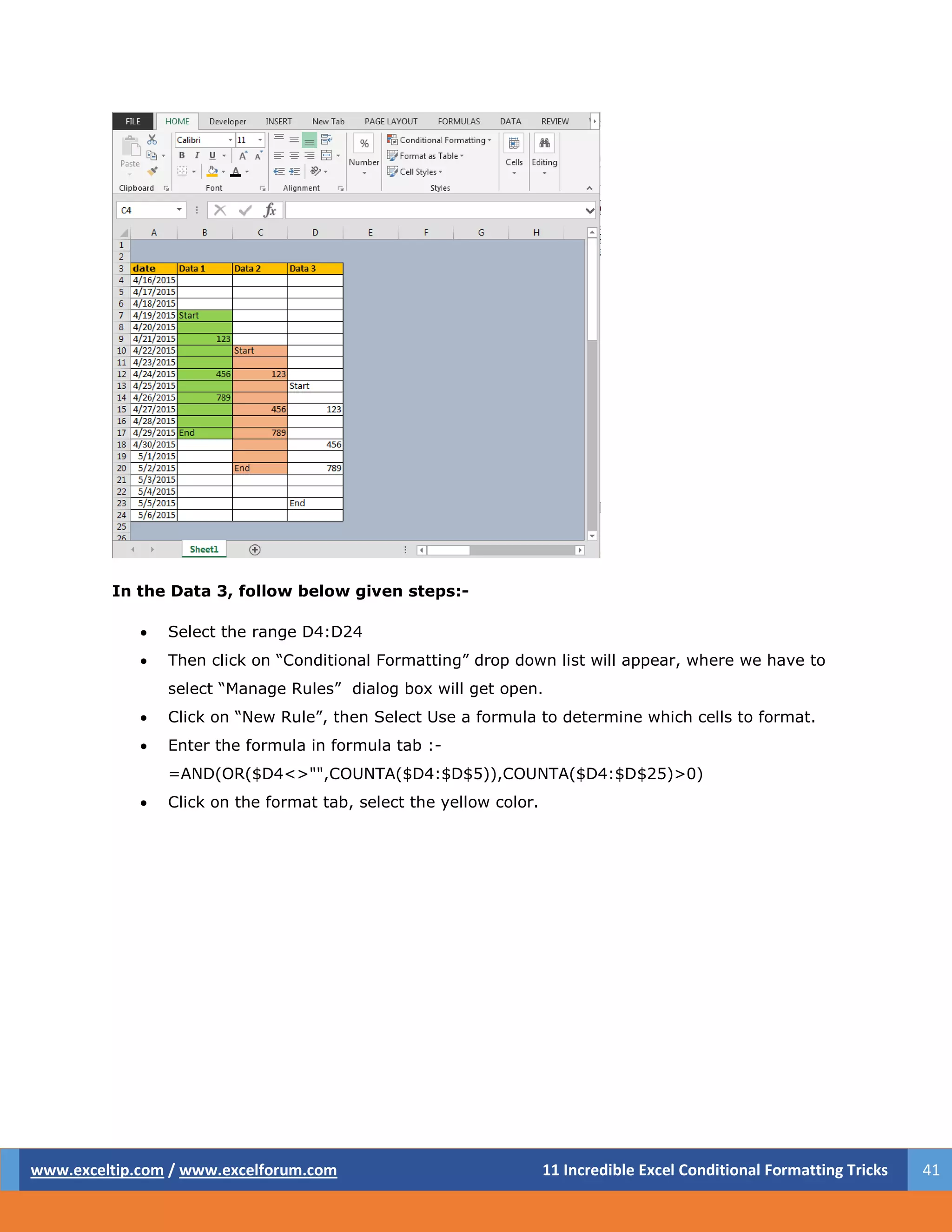
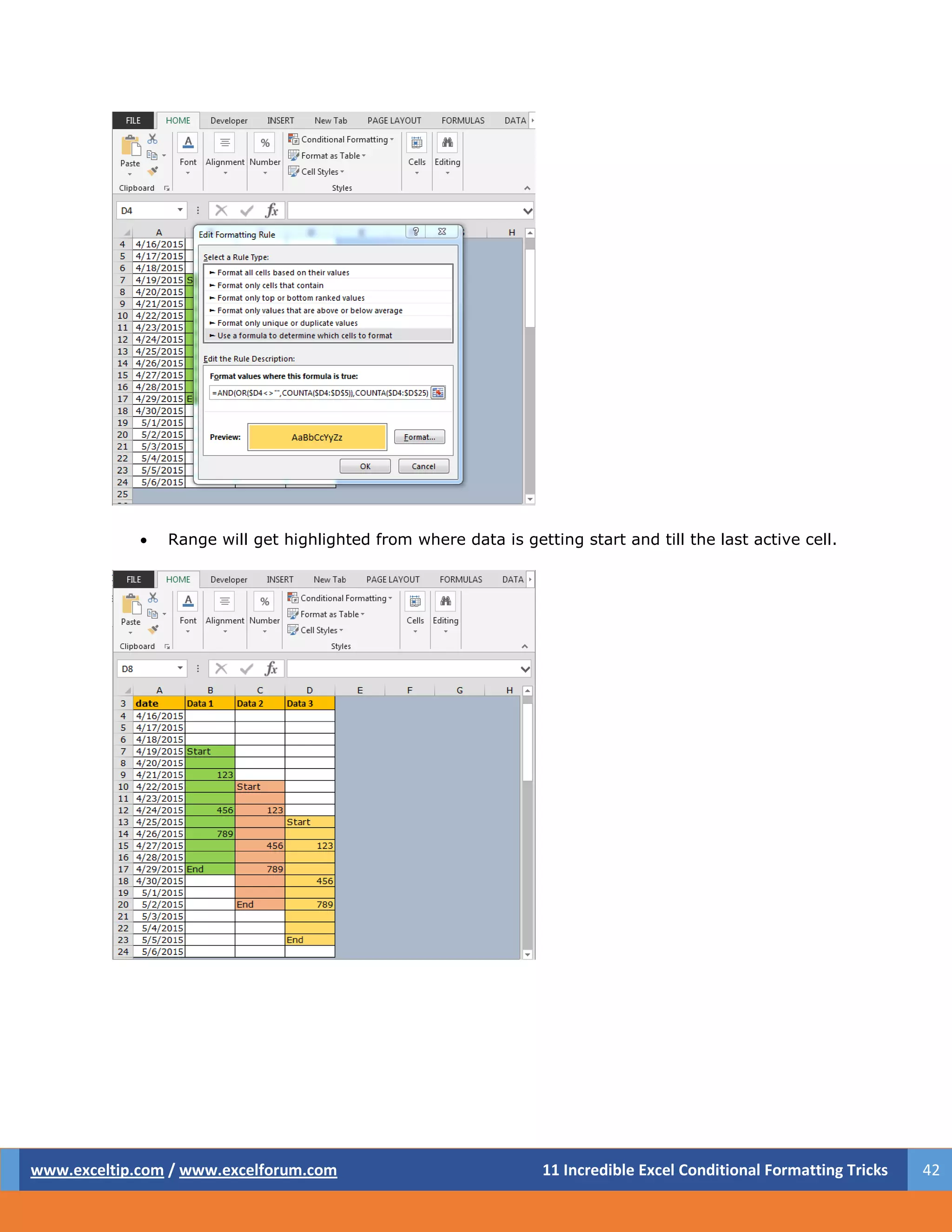
have value in the range then we can use Conditional Formatting by describing the formula
to highlight the values.
There are lot ways to use “Conditional Formatting” in our data. We can use it to show the
numbers in increasing and decreasing order, to specific Value, to specific numbers, to
specific date etc. Also we can highlight the cells by fill the color in cell, by change the font
color, by using the data bars, color scales, icon sets.

What we are going to learn in this book?
1. Conditional Format Based on Dates.......................................................................…………4
2. Find Occurrence of Text in a Column through Conditional formatting..............................8
3. How to highlight a row on the basis of cell…………………………………………………………………..11
4. Compare 2 Columns and Return Fill Red if is different.....................................................14
5. How to check the row and then highlight the first cell of the row...................................18
6. Highlight Cells Tomorrow Excluding Weekend.........................................................………22
7. Conditional Formatting to Mark Dates on a Calendar......................................................27
8. Counting the Length of Characters in a Cell before a Particular Character......................32
9. Highlight the Top 10 Sales through Conditional Formatting………………………………………...38
10. Conditional Formatting for Pivot Tables……………………………………………………………………….43
11. Conditional Format Between First and Last Non-Blank Cells…………………………………………46

Conditional Format Based on Dates
http://www.excelforum.com/excel-formulas-and-functions/1077036-conditional-format-
based-on-dates.html
Question:-
I have been searching but i cant solve my issue, I want to conditional format a cell that will
be either, Green, Yellow or red depending on the date.
 If the date I enter in Cell C2 is more than 60 days from today the cell should be
green.
 If the date is less than 60 days from today the cell should be yellow.
 If the cell is less than 30 days from today the cell should be red
This is for drivers licence dates, i want to be alerted when they are 60 days from the
expiration etc
Topic 1:

To put the “Conditional Formatting” follow below given steps:-
 Select the range, where we want to do “Conditional Formatting”.
 When we will click on “Conditional Formatting” drop down list will appear, where we
have to select “Manage Rules” dialog box will get open.
 Where we have to click on “New Rule”, New Formatting Rule dialog box will get
appear, click on Use a formula to determine which cells to format.
 First we will apply the “Conditional Formatting” for (If the date I enter in Cell C2 is
more than 60 days from Today).
 Enter the formula =AND(C2<>"", C2>TODAY()+60).
 Click on Format and select the green color.
 Again we will click on “New Rule”, New Formatting Rule dialog box will get appear,
click on Use a formula to determine which cells to format.
 Now will enter the formula for (If the date is less than 60 days from today).
 Enter the formula =AND(C2<>"", C2<TODAY()-30)
 Click on Format and select the Yellow color.

 Again we will click on “New Rule”, New Formatting Rule dialog box will get appear,
click on Use a formula to determine which cells to format.
 In last we will enter the formula for (If the cell is less than 30 days from today).
 Enter the formula =AND(C2<>"", C2>TODAY()-60)
 Click on Format and select the Red color.

 Click on Apply and then on ok.

Find Occurance of Text in a Column through Conditional formatting
http://www.excelforum.com/excel-general/1076335-find-occurance-of-text-in-a-column.html
Question:-
I have 2 workbooks. In workbook (1), I have a column with a few thousand store names. In
workbook (2), I have a column with a few hundred store names. The store names are not
identical but have the following unique words/numbers: ABC123 etc. I want to identify if a
store in workbook (2) exists in workbook (1). I have attached a sample file.
In Workbook 2, we have 2 columns, in Which column A contains only series number and in
Column B we will get the whole product name through series number, which is common in
both data.
To return the whole product number in workbook 2 use below given formula:-
 =IFERROR(IF(G2="","",INDEX($B$2:$B$8,MATCH("*"&G2&"*",$A$2:$A$8,0))),"")
Topic 2:

 Press Enter.
 Copy the same formula and paste in the range.
To put the “Conditional Formatting” follow below given steps:-
 When we will click on “Conditional Formatting” drop down list will appear, where we
have to select “Manage Rules” dialog box will get open.
 =COUNTIF($H$2:$H$8,A2)>0

 Click on Apply and then on ok.

How to Highlight a row on the basis of Cell
http://www.excelforum.com/excel-programming-vba-macros/1076156-highlighting-a-row-filling-a-row-
automatically-with-a-different-color.html
Question:-
I want to highlight the row which shows the maximum GPA. It has to be happened
automatically at the end of GPA calculation. Here it is 21st row with a maximum value of
4.0.
In this query users want to highlight the row with the color on the basis of Maximum
number in the cell.
In column AA whatever cell is having the maximum DGPA that rows should be highlighted
with color.
Topic 3:

To resolve this query our expert has given the “Conditional Formatting” option. Now let’s
see how we can do it through Conditional Formatting:-
 Select the range DGPA AA8:AA46.
 Then click on “Conditional Formatting” drop down list will appear, where we have to
select “Manage Rules” dialog box will get open.
 =$AA8=MAX($AA$15:$AA$53)
 Row will get highligt with the selected color.

This is the way we can highlight the row on the basis of cell value.

Compare 2 Colomns and return fill red if it is different
http://www.excelforum.com/excel-general/1076097-compare-2-colomns-and-return-fill-red-if-is-
different.html
Question:-
I want to compare 2 columns( A coulomn and B columns ) if data in columns B is different i
want to change to red color.
I ask you a simple version for my problem but the problem is little more difficult I want to
compare a list of coulomns A and B for example P.12242 with R1112242900 ; 12242 is
common number
Topic 4:

In the above mentioned query user want to compare two columns, in which he wants where
the cells are not same in the both column that should be highlighted with the Red color.
Our Excel expert has given very nice reply and resolve his problem. Let’s see how we can do
compare two columns through Conditional Formatting.
 Select the both columns Column A and B.
 =MID($A2,3,5)<>MID($B2,4,5)
 Click on ok.
 Then Click on Apply, and ok.

If the cells will not matched in both of the columns then it will get highlighted with the Red
color.
This the way we can use the Conditional Formatting to compare the two columns with each
other.

How to check the row and then highlight the first cell of the row
http://www.excelforum.com/excel-formulas-and-functions/1075698-conditional-formating.html
Question:-
I have created task completed YES/NO excel sheet. I have used conditional formatting as you
can see, YES turns Green, No turns Red. There are task for 5 Stores.I need to
use conditional formatting in cell A2:A11 with following condition:
If any cell in particular task is incomplete (NO) then highlight cell in column A RED otherwise
turn Green. Basically looking at the data cell A2,A5,A8 needs to turn green and rest needs
to turn Red
To highlight the cells on the basis of rows, follow below given steps:-
 Select the both columns Column A and B.
Topic 5:

 To highlight the cell for “YES” enter the formula.
 =COUNTIF(B2:F2,"Yes")=5
 Click on Format and select the Green color.
 Click on ok.
 To highlight the cell for “NO” enter the formula.
 =COUNTIF(B2:F2,"Yes")=5

 Click on ok.
 Then click on Apply, and ok.

Highlight Cells Tomorrow Excluding Weekend
http://www.excelforum.com/excel-general/1077310-highlight-cells-tomorrow-
excluding-weekend.html
Question:-
I have dates entered manually down the C column and i use the standard highlight rule to
color the cells i.e. today. Tomorrow and Yesterday. Now my issue is come Friday in the
week I wish to have Mondays date highlighted as Tomorrow so it has excluded the
weekend. The standard conditional formatting for when date occurs won’t work in this
instance and I have tried at least 20 formulas from forums etc.
What am I doing wrong? Or is there a simpler way? I just wish it to not count any weekends
and make Friday 1 and Monday the day after so it will highlight as if it was tomorrow
Topic 6:

To resolve this problem, Our Expert has used the combinations of formulas:- “TODAY”,
“WORKDAY” and “IF” functions.
“TODAY” function will help to return the today date.
“IF” function will help to check the condition and then will perform accordingly.
“WORKDAY” function will help to return the serial number of the date before or after a
specified number of workdays.
To highlight the tomorrow date we will use the combination of formula in conditional
formatting option, follow below given steps:-
 Go to Home tab, select “Conditional Formatting” under the Styles group and select
“New Rule”.

 Select the range of Date.
 “New Formatting Rule” dialog box will get appear.
 Click on “Use a formula to determine which cells to format”.
 Then enter the formula:- =IF(TODAY()+1=WORKDAY(B2,0,2),TODAY()+1,"")
 Tomorrow date will get highlighted, but if there is weekend tomorrow then it will not
be highlighted.

Conditional Formatting to Mark Dates on a Calendar
http://www.excelforum.com/excel-formulas-and-functions/1077491-conditional-formatting-to-mark-
dates-on-a-calendar.html
Question:-
I have a calendar that I want to mark the dates as per the listed Date Criteria. I thought
conditional formatting would be the best way, however can't seem to find a way.
Following is the list of start & finish dates in column A & B
We want conditional formatting to highlight dates that matches Dates Criteria in column D;
refer below snapshot
Topic 7:

We need to follow the below steps:
 Select range A2:B10
 Click on Home ribbon; from Styles group select Conditional Formatting or use
shortcut key ALT + O + D
 Click on New Rule
 Select “Use a formula to determine which cells to format”
 Enter the formula as =IF(OR(A2=$D$2,A2=$D$3,A2=$D$4),TRUE)

 Click on Format & select the color of your choice
 Click on Ok button twice; we will get the require result

Counting the Length of Characters in a Cell before a Particular Character
http://www.excelforum.com/excel-general/818753-counting-the-length-of-characters-in-a-
cell-before-a-particular-character.html
Question:-
I am trying to highlight cells that contain an X number of characters before the - sign. For
e.g... Let’s say I have a list like this:
12-2929
0993-2929
00992-2939
10-2929
from the above list I would like to highlight cells that contain 2 characters before the dash,
i.e., 12-2929 and 10-2929. I was wondering, what would be the best way of doing this via
conditional formatting or using the Len formula in combination with another formula?
Topic 8:

 Select the range & press ALT + O + D
 New Formatting Rule window will be pop up
 Enter the formula as =FIND("-",A1)-1=2

 Click on Format & fill the color of your choice.
 You will get the desired result.

Highlight the Top 10 Sales through Conditional Formatting
http://www.excelforum.com/showthread.php?t=1077896&p=4047123#post4047123
Question:-
I have a list of sales in which I have sales amount. I want to highlight the top sales on the
basis of sales amount, how I can do it through "Conditional Formatting".
Topic 9:

Follow below given steps to highlight the top 10 sales:-
 Select the range A2:B21 & press ALT + O + D shortcut key to open Conditional Formatting Rules
Manager.
 Click on New Rule; New Formatting Rule window will appear

 In “Format values where this formula is true” enter the following formula
 =$B2>=LARGE($B$2:$B$21,10)
 Click on Format & pick the color of your choice.
 Click on Ok button twice you will see Conditional Formatting gets applied on the selected range
of cells refer below snapshot

In this way we can highlight top 10 or any value from large amount of data using conditional formatting
feature of excel.

Conditional Formatting for Pivot Tables
http://www.excelforum.com/excel-general/1077420-conditional-formatting-for-pivot-
tables.html
Question:-
I have months in my pivot table and years (in the row column). How can I set up
conditional formatting JUST on the month values?
We want to highlight the maximum immpression in the range in “Pivot Table”.
Follow below given steps:-
 Select the range H3:J3.
 Select “This PivotTable” from the drop down list of Show formatting rules for:-
Topic 10:

 Click on “New Rule”, then define the range where we want to apply the rule.
 Select value:- Top 1 and then format it with Green color.
 Maximum number will get highlighted in the list.

Note:- Whenever we will referesh the pivot table after add the data in table, conditional
formatting will be applicable accordingly

Conditional Format Between First and Last Non-Blank Cells
http://www.excelforum.com/showthread.php?t=1077928&p=4047438#post4047438
Question:-
I need to conditionally format cells that are between first non-blank and last non-blank in
column wise...
User want to highlight the range from the first non blank cell till the last non blank cell in
the columns of data 1, 2, and 3.
In the Data 1, follow below given steps:-
Topic 11:

 Select the range B4:B24
 Click on “New Rule”, then Select Use a formula to determine which cells to format.
 Enter the formula in formula tab :-
=AND(OR($B4<>"",COUNTA($B4:$B$5)),COUNTA($B4:$B$25)>0)
 Click on the format tab, select the green color.

 Range will get highlighted from where data is getting start and till the last active cell.

 Select the range C4:C24
=AND(OR($C4<>"",COUNTA($C4:$C$5)),COUNTA($C4:$C$25)>0)
 Click on the format tab, select the Orange color.

 Select the range D4:D24
=AND(OR($D4<>"",COUNTA($D4:$D$5)),COUNTA($D4:$D$25)>0)
 Click on the format tab, select the yellow color.

Download 11-incredible-excel-conditional-formatting-tricks

Recommended

Recommended

More Related Content

What's hot

What's hot (20)

Similar to Download 11-incredible-excel-conditional-formatting-tricks

Similar to Download 11-incredible-excel-conditional-formatting-tricks (20)

Recently uploaded

Recently uploaded (20)

Download 11-incredible-excel-conditional-formatting-tricks