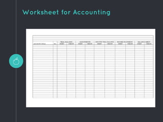
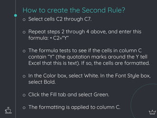
An Excel worksheet is a single spreadsheet containing cells organized in rows and columns. Worksheets can be used for accounting, classroom exercises, and other tasks. The document discusses how to format worksheets by applying borders, changing text colors and alignment, adding cell shading, and using conditional formatting. Conditional formatting allows rules to highlight important information, such as formatting cells red and bold if they contain future dates or formatting cells green and bold if they contain a "Y".

1. Worksheets

2. What is a worksheet?
o An Excel worksheet is a single spreadsheet that contains
cells organized by rows and columns.
o A paper for recording work done or in progress.
o In accounting a worksheet often refers to a loose leaf piece
of stat from a columnar pad.
o In the classroom setting worksheets usually refer to a loose
sheet of paper with questions or exercises

3. o Excel Worksheet

4. Worksheet for Accounting

5. “
How to Format Worksheets?
1. Apply Cell Border
o Select the cell or range of cells that you want to
add a border to.
o On the Home tab, in the Font group, click the
arrow next to Borders , and then click the border
style that you want.

6. 2. Change Text Color and Alignment
o Select the cell or range of cells that contain (or will
contain) the text that you want to format.
o To change the color of text in the selected cells, click
the arrow next to Font Color , and then
under Theme Colors or Standard Colors, click the
color that you want to use.
o To change the alignment of the text in the selected
cells, on the Home tab, in the Alignment group, click
the alignment option that you want.
How to Format Worksheets?

7. How to Format Worksheets?
3. Apply Cell Shading
o Select the cell or range of cells that you
want to apply cell shading to.
o On the Home tab, in the Font group, click
the arrow next to Fill Color , and then
under Theme Colors or Standard Colors,
click the color that you want.

8. How to create the First Rule?
◦Select cells A2 through A7. Do this by dragging
from A2 to A7.
◦Then, click Home > Conditional Formatting > New
Rule.
◦In the New Formatting Rule dialog box, click Use a
formula to determine which cells to format.
◦Under Format values where this formula is true,
type the formula: =A2 TODAY ()

9. What is Conditional Formatting?
o Conditional formatting quickly highlights
important information in a spreadsheet.
o But sometimes the built-in formatting rules
don’t go quite far enough.
o Adding your own formula to a conditional
formatting rule gives it a power boost
o It helps you do things, the built-in rules can’t
do.

10. How to create the First Rule?
The formula uses the TODAY function to see if the
dates in column A are greater than today (in the
future). If so, the cells are formatted.
◦Click Format.
◦In the Color box, select Red. In the Font Style box,
select Bold.
◦Click OK until the dialog boxes are closed.
◦The formatting is applied to column A.

11. DidYouKnowThat?
o You can actually play tetris by the use of MS
Excel.
o MS Excel can also be used as Sudoku
Generator and Solver
o A Traditional Slide Puzzle can also be played
here by the use of macros

12. How to create the Second Rule?
o Select cells C2 through C7.
o Repeat steps 2 through 4 above, and enter this
formula: =C2="Y“
o The formula tests to see if the cells in column C
contain “Y” (the quotation marks around the Y tell
Excel that this is text). If so, the cells are formatted.
o In the Color box, select White. In the Font Style box,
select Bold.
o Click the Fill tab and select Green.
o The formatting is applied to column C.

13. PRESENTAION BY: Naomi Faith