Richard Giles Walters
Conditional Formatting
and Conditional
Formulas
2
RICHARD GILES WALTERS
CONDITIONAL
FORMATTING AND
CONDITIONAL
FORMULAS
3
Conditional Formatting and Conditional Formulas
1st
edition
© 2021 Richard Giles Walters & bookboon.com
ISBN 978-87-403-3864-5
CONDITIONAL FORMATTING AND
CONDITIONAL FORMULAS Contents
4
CONTENTS
About the Author 5
Liability and warranty 7
Introduction 8
1	
What is Conditional Formatting 9
1.1 Highlight Cell Rules 9
1.2 Top/Bottom Rules 48
1.3 Data Bars 66
1.4 Colour Scales 77
1.5 Icon Sets 81
1.6 New Rule 87
1.7 Manage Rules and Editing Rules 88
1.8 Clearing Conditional Formatting 91
1.9	
Multiple Conditional Formatting Example (Highlight Cell Rules) 92
2	
Conditional Formatting Formulas 97
2.1	
Creating Conditional Formulas and Cell Referencing 97
2.2	
Conditional Formula signs and using signs in formulas 101
2.3 Applying Formula Formatting 102
2.4 Testing Conditional Formatting Formulas 105
2.5	
Controlling and Ordering Formula Formatting (“Stop If True”) 111
2.6 Managing and Editing Formula Results 115
2.7 Hiding “Zero” values and/or percentages 120
2.8 Conditional Formatting Formula Examples 122
Table of Figures 138
CONDITIONAL FORMATTING AND
CONDITIONAL FORMULAS About the Author
5
ABOUT THE AUTHOR
My name is Richard Giles Walters, and I am a qualified teacher (Cert/Ed) with a vast
experience in training Microsoft (MS) Office applications. I constantly look at ways I can
improve myself and my knowledge in the use of MS Office and I am qualified as a Microsoft
Office Specialist (MOS) Expert. I am an MS Office enthusiast and a firm believer in how
the different MS Office applications can be used effectively, to improve business productivity.
I have written the book “Conditional Formatting and Conditional Formulas” using my
training experience and experience in using MS Excel, to take the reader on a visual journey
through the use of colour settings and applying colour to MS Excel information. The book
is very visual and designed to take the reader through a “Step by Step” learning process with
multiple demonstration examples, to provide the reader with different ideas in how colour
can be applied to MS Excel information for business or personal needs.
I am an experienced book author and have produced other MS Office publications, both
e-books and paperback books and these are available for purchase through NILC Training
(www.nilc.co.uk) and Amazon. I also produce online training videos covering MS Excel and
many other MS Office applications which are available for resale through my online training
partner, NILC Training (www.nilc.co.uk). My online training partner NILC Training also
have a YouTube Channel (NILC Training) and I have produced many online training videos
covering multiple MS Office application areas including MS Excel, which are available on
their YouTube Channel.
CONDITIONAL FORMATTING AND
CONDITIONAL FORMULAS About the Author
6
I deliver MS Office training on a regular basis where I deliver both classroom training and
online training. I can be contacted for any training requirements using the contact details
provided below.
I enjoyed producing this book for Bookboon and I hope the book is a useful resource to
all readers and fellow MS Excel enthusiasts.
Contact Information:
 		 richard.walters@key-strokes.co.uk
		 www.linkedin.com/in/richard-walters-59047127
NILC Training YouTube Channel
Website: www.key-strokes.co.uk
Video Sales: www.nilc.co.uk
Book Sales: Bookboon, Amazon and NILC Training (www.nilc.co.uk)
CONDITIONAL FORMATTING AND
CONDITIONAL FORMULAS Liability and warranty
7
LIABILITY AND WARRANTY
Microsoft and Microsoft (R) Excel, Microsoft (R) Access, Microsoft (R) PowerPoint, Microsoft
(R) SharePoint, Microsoft (R) Outlook and Microsoft (R) Word are trademarks or registered
trademarks of the Microsoft Corporation. All other trademarks are the property of their
respective companies. All trademarks are used with the permission of Microsoft.
Most of the product names for hardware and software, as well as company names and
company logos, that are mentioned in this e-book are registered trademarks and should
be viewed as such. Concerning product names, the publisher fundamentally follows the
notations of the various manufacturers.
All graphics, screenshots and texts provided by the author are used in accordance with
Microsoft requirements for permitted use (use of copyrighted content from Microsoft,
last update on 29th
of March in 2015 at https://www.microsoft.com/en-us/legal/copyright/
permissions)
All procedures and programs described in this e-book serve teaching and learning purposes.
The author assumes no liability or guarantee for the topicality, correctness, completeness or
quality of the information provided.
Liability claims against the author relating to material or immaterial damage caused by
the use or non-use of the information provided as well as using incorrect and incomplete
information are fundamentally excluded, provided that the author has no proven intentional
or grossly negligent fault. All persons and exercise situations in this e-book are fictitious and
do not show any deliberately intended resemblance to living or dead persons.
CONDITIONAL FORMATTING AND
CONDITIONAL FORMULAS Introduction
8
INTRODUCTION
In the modern workplace there is a great need to review and report on specific information
stored in Microsoft (MS) Excel. This is often time consuming if the right techniques and
tools are not used and can lead to company information reporting delays. The use of colour
has major advantages in analysing data and trends and reporting on these areas in MS
Excel. The use of colour in MS Excel to manage information is referred to as “Conditional
Formatting” and this skill can greatly aid data analysis, reviewing data and can save vast
amounts of time when performing these tasks.
The book covers in detail the area of “Conditional Formatting”, reviewing areas like
“Highlight Cell Rules”, “Icon Sets”, “Highlighting Duplicate Values” and “Colour Scales”.
There are detailed explanations on how to apply colour settings and also how to modify
colour settings through the use of “Conditional Formatting”.
As well as covering “Conditional Formatting” in detail the book also covers the use of
“Conditional Formatting Formulas”. This area of “Conditional Formatting” is very powerful
and can be used to apply colour settings to information in MS Excel, using a variety of
Excel Functions including, IF, And, Or, Sum, Average and Countifs. The book emphasises
the importance of “Testing” formulas in MS Excel then copying the tested formulas as
“Conditional Formatting Formulas”. The book also makes the reader aware of the importance
of “True” and “False” results when testing and using “Conditional Formatting Formulas”.
There are many formula examples demonstrated in the book including Data Comparison
formulas and Target Setting formulas.
CONDITIONAL FORMATTING AND
CONDITIONAL FORMULAS What is Conditional Formatting
9
1	
WHAT IS CONDITIONAL
FORMATTING
Microsoft (MS) Excel spreadsheet information can often be difficult to interpret, and
this can be for a variety of reasons. The design of the spreadsheet might not have been
designed effectively and due to the design, the spreadsheet may not be “fit for purpose”.
Many spreadsheets are often populated with vast amounts of business information which
can be difficult to read, for data trends and data changes. There could be data changes from
“Month to Month” or “Quarter by Quarter” and this information can be difficult to review
and analyse. By using colour to highlight information against set analytical conditions, this
can make reviewing large amounts of information much more manageable.
Conditional Formatting in MS Excel is the use of colour and coloured symbols to highlight
information against set analytical conditions. Information in MS Excel is highlighted, and
colour is applied to the highlighted data range, and this is how Conditional Formatting
works.
An example of Conditional Formatting is demonstrated below, where colour is applied to
a range of information. The Conditional Formatting demonstrated below, demonstrates the
use of “Data Bars” and how they can be used to monitor progress against set targets. In
the example below “Data Bars” are applied to the cell range cell K2 to cell K21 and the
cell range cell M2 to cell M21.
Figure 1 – Conditional Formatting Example
1.1 HIGHLIGHT CELL RULES
One of the biggest areas of Conditional Formatting is an area called “Highlight Cell Rules”
and this area is covered in great detail. The following areas are demonstrated under the area
“Highlight Cell Rules”:
CONDITIONAL FORMATTING AND
CONDITIONAL FORMULAS What is Conditional Formatting
10
• Greater Than
• Less Than
• Between
• Equal To
• Text That Contains
• Date Occurring
• Duplicate Rules
• More Rules (including Greater Than or Equal to and Less Than or Equal to)
1.1.1 GREATER THAN
Information is tested for the Conditional Formatting area “Greater Than”, when highlighted
spreadsheet information is either entered as a numerical or text entry. The information
entered is then tested using Conditional Formatting, for either numerical values greater
than a certain value or text entries greater than a certain letter of the alphabet.
Example Scenario – Step by Step
Format all theTurnover figures which are Greater Than £15,000 with “Green font formatting”.
The original information is demonstrated below:
Figure 2 - Greater Than (A)
The Turnover information in the cell range cell I2 to cell I21 is highlighted and the “Greater
Than” option is selected from the “Highlight Cell Rules” area on the “Home Tab”.
CONDITIONAL FORMATTING AND
CONDITIONAL FORMULAS What is Conditional Formatting
11
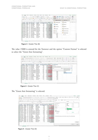
Figure 3 - Greater Than (B)
The value 15000 is entered for the Turnover and the option “Custom Format” is selected
to select the “Green font formatting”.
Figure 4 - Greater Than (C)
The “Green font formatting” is selected.
Figure 5 - Greater Than (D)
CONDITIONAL FORMATTING AND
CONDITIONAL FORMULAS What is Conditional Formatting
12
The “OK” button for the “Greater Than” option is selected to apply the “Green font
formatting” to the highlighted Turnover information.
Figure 6 - Greater Than (E)
The “Green font formatting” has now been applied to the Turnover information for the
cell range cell I2 to cell I21.
Figure 7 - Greater Than (F)
1.1.2 LESS THAN
Information is tested for the Conditional Formatting area “Less Than”, when highlighted
spreadsheet information is either entered as a numerical or text entry. The information
entered is then tested using Conditional Formatting, for either numerical values less than
a certain value or text entries less than a certain letter of the alphabet.
CONDITIONAL FORMATTING AND
CONDITIONAL FORMULAS What is Conditional Formatting
13
Example Scenario – Step by Step
Format all the Turnover figures which are Less Than £15,000 with “Red font formatting”.
The original information is demonstrated below:
Figure 8 - Less Than (A)
The Turnover information in the cell range cell I2 to cell I21 is highlighted and the “Less
Than” option is selected from the “Highlight Cell Rules” area on the “Home Tab”.
Figure 9 - Less Than (B)
The value 15000 is entered for the Turnover and the option “Custom Format” is selected
to select the “Red font formatting”.
CONDITIONAL FORMATTING AND
CONDITIONAL FORMULAS What is Conditional Formatting
14
Figure 10 - Less Than (C)
The “Red font formatting” is selected.
Figure 11 - Less Than (D)
The “OK” button for the “Less Than” option is selected to apply the “Red font formatting”
to the highlighted Turnover information.
CONDITIONAL FORMATTING AND
CONDITIONAL FORMULAS What is Conditional Formatting
15
Figure 12 - Less Than (E)
The “Red font formatting” has now been applied to the Turnover information for the cell
range cell I2 to cell I21.
Figure 13 - Less Than (F)
1.1.3 BETWEEN
Information is tested for the Conditional Formatting area “Between”, when highlighted
spreadsheet information is either entered as a numerical or text entry. The information
entered is then tested using Conditional Formatting, for either numerical values between
two certain values or text entries between two letters of the alphabet.
CONDITIONAL FORMATTING AND
CONDITIONAL FORMULAS What is Conditional Formatting
16
Example Scenario – Step by Step
Format all the Sales Quantity figures which are Between 1000 and 5000 with “Red font
formatting”.
The original information is demonstrated below:
Figure 14 - Between (A)
Discover our eBooks
on Leadership Skills
and hundreds more
Download now
CONDITIONAL FORMATTING AND
CONDITIONAL FORMULAS What is Conditional Formatting
17
The Sales Quantity information in the cell range cell G2 to cell G21 is highlighted and
the “Between” option is selected from the “Highlight Cell Rules” area on the “Home Tab”.
Figure 15 - Between (B)
The values are entered between 1000 and 5000 and the option “Custom Format” is selected
to select the “Red font formatting”.
Figure 16 - Between (C)
The “Red font formatting” is selected.
CONDITIONAL FORMATTING AND
CONDITIONAL FORMULAS What is Conditional Formatting
18
Figure 17 - Between (D)
The “OK” button for the “Between” option is selected to apply the “Red font formatting”
to the highlighted Sales Quantity information.
Figure 18 - Between (E)
The “Red font formatting” has now been applied to the Sales Quantity information for the
cell range cell G2 to cell G21.
CONDITIONAL FORMATTING AND
CONDITIONAL FORMULAS What is Conditional Formatting
19
Figure 19 - Between (F)
1.1.4 EQUAL TO
Information is tested for the Conditional Formatting area “Equal To”, when highlighted
spreadsheet information is either entered as a numerical or text entry. The information
entered is then tested using Conditional Formatting, for either numerical values equal to a
certain value or text entries equal to a certain letter of the alphabet.
Example Scenario – Step by Step
Format the Product information which are equal to “Baseball” products with “Green Cell
formatting”.
The original information is demonstrated below:
CONDITIONAL FORMATTING AND
CONDITIONAL FORMULAS What is Conditional Formatting
20
Figure 20 - Equal To (A)
The Product information in the cell range cell E2 to cell E21 is highlighted and the “Equal
To” option is selected from the “Highlight Cell Rules” area on the “Home Tab”.
Figure 21 - Equal To (B)
A text value is entered equal to the word “Baseballs” and the option “Custom Format” is
selected to select the “Green Cell formatting”.
CONDITIONAL FORMATTING AND
CONDITIONAL FORMULAS What is Conditional Formatting
21
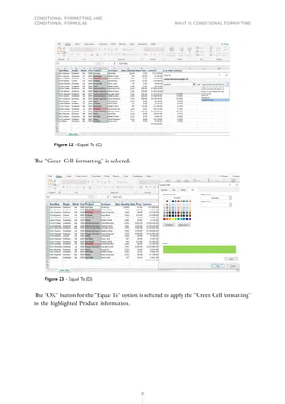
Figure 22 - Equal To (C)
The “Green Cell formatting” is selected.
Figure 23 - Equal To (D)
The “OK” button for the “Equal To” option is selected to apply the “Green Cell formatting”
to the highlighted Product information.
CONDITIONAL FORMATTING AND
CONDITIONAL FORMULAS What is Conditional Formatting
22
Figure 24 - Equal To (E)
The “Green Cell formatting” has now been applied to the Product information for the cell
range cell E2 to cell E21.
Figure 25 - Equal To (F)
1.1.5 TEXT THAT CONTAINS
Information is tested for the Conditional Formatting area “Text That Contains”, when
highlighted spreadsheet information is entered as a text entry. The information entered is then
tested using Conditional Formatting, for text entries which contain a certain alphabetical
letter or specific word(s).
CONDITIONAL FORMATTING AND
CONDITIONAL FORMULAS What is Conditional Formatting
23
Example Scenario – Step by Step
Format the Product information which contains any “machine” products with “Green Cell
formatting”.
The original information is demonstrated below:
Figure 26 - Text That Contains (A)
The Product information in the cell range cell E2 to cell E21 is highlighted and the “Text
That Contains” option is selected from the “Highlight Cell Rules” area on the “Home Tab”.
Figure 27 - Text That Contains (B)
The text value “machine” is entered, and the option “Custom Format” is selected to select
the “Green Cell formatting”.
CONDITIONAL FORMATTING AND
CONDITIONAL FORMULAS What is Conditional Formatting
24
Figure 28 - Text That Contains (C)
The “Green Cell formatting” is selected.
Figure 29 - Text That Contains (D)
The “OK” button for the “Text That Contains” option is selected to apply the “Green Cell
formatting” to the highlighted Product information.
CONDITIONAL FORMATTING AND
CONDITIONAL FORMULAS What is Conditional Formatting
25
Figure 30 - Text That Contains (E)
The “Green Cell formatting” has now been applied to the Product information for the cell
range cell E2 to cell E21.
Figure 31 - Text That Contains (F)
1.1.6 DATE OCCURRING
Information is tested for the Conditional Formatting area “Date Occurring”, when highlighted
spreadsheet information is entered as a date entry. The information entered is then tested
using Conditional Formatting, for certain date requirements.
CONDITIONAL FORMATTING AND
CONDITIONAL FORMULAS What is Conditional Formatting
26
Example Scenario – Step by Step
Format all the sales for the last month with “Green Cell formatting”. For this example,
today’s date is 08/06/2021.
The original information is demonstrated below:
Figure 32 - Date Occurring (A)
Discover our eBooks on
Communication Skills
and hundreds more
Download now
CONDITIONAL FORMATTING AND
CONDITIONAL FORMULAS What is Conditional Formatting
27
The Date of Sale information in the cell range cell A2 to cell A21 is highlighted and the “A
Date Occurring” option is selected from the “Highlight Cell Rules” area on the “Home Tab”.
Figure 33 - Date Occurring (B)
The date option “Last month” is selected, and the option “Custom Format” is selected to
select the “Green Cell formatting”.
Figure 34 - Date Occurring (C)
The “Green Cell formatting” is selected.
CONDITIONAL FORMATTING AND
CONDITIONAL FORMULAS What is Conditional Formatting
28
Figure 35 - Date Occurring (D)
The “OK” button for the “Date Occurring” option is selected to apply the “Green Cell
formatting” to the highlighted Date of Sale information.
Figure 36 - Date Occurring (E)
The “Green Cell formatting” has now been applied to the Date of Sale information for the
cell range cell A2 to cell A21.
CONDITIONAL FORMATTING AND
CONDITIONAL FORMULAS What is Conditional Formatting
29
Figure 37 - Date Occurring (F)
1.1.7 DUPLICATE VALUES
Information is tested for the Conditional Formatting area “Duplicate Values”, when
spreadsheet information is entered. The information entered is then tested using Conditional
Formatting, for duplicate entries.
Example Scenario – Step by Step
Format all duplicate staff number entries with “Red Cell formatting”.
The original information is demonstrated below:
Figure 38 - Duplicate Values (A)
CONDITIONAL FORMATTING AND
CONDITIONAL FORMULAS What is Conditional Formatting
30
The Staff Number information in the cell range cell A2 to cell A11 is highlighted and the
“Duplicate Values” option is selected from the “Highlight Cell Rules” area on the “Home Tab”.
Figure 39 - Duplicate Values (B)
The option “Duplicate” is selected, and the option “Custom Format” is selected to select
the “Red Cell formatting”.
Figure 40 - Duplicate Values (C)
The “Red Cell formatting” is selected.
CONDITIONAL FORMATTING AND
CONDITIONAL FORMULAS What is Conditional Formatting
31
Figure 41 - Duplicate Values (D)
The “OK” button for the “Duplicate Values” option is selected to apply the “Red Cell
formatting” to the highlighted Staff Number information.
Figure 42 - Duplicate Values (E)
The “Red Cell formatting” has now been applied to the Staff Number information for the
cell range cell A2 to cell A11.
CONDITIONAL FORMATTING AND
CONDITIONAL FORMULAS What is Conditional Formatting
32
Figure 43 - Duplicate Values (F)
1.1.8 MORE RULES
Information is tested for the Conditional Formatting area “More Rules”, when numerical
or text spreadsheet information is entered and highlighted. The Conditional Formatting
option “More Rules” which is located in the “Highlight Cell Rules” area of Conditional
Formatting, provides extra useful formatting options. These options include testing highlighted
information with the rules “Greater Than or Equal To” and “Less Than or Equal To”, as
well as other useful tests on blank cells. Some of the different options under the “More
Rules” area, will now be demonstrated.
Greater Than or Equal To Example Scenario – Step by Step
Format all the figures which are Greater Than or Equal To 14% in the “% of Total Turnover”
information, with green cell formatting.
The original information is demonstrated below:
Figure 44 - Greater Than or Equal To (A)
CONDITIONAL FORMATTING AND
CONDITIONAL FORMULAS What is Conditional Formatting
33
The Percentage (%) information in the cell range cell J2 to cell J21 is highlighted and the
“More Rules” option is selected from the “Highlight Cell Rules” area on the “Home Tab”.
Figure 45 - Greater Than or Equal To (B)
The option “Greater Than or Equal To” is selected from the list of options from the “Format
only cells than contain” area, as demonstrated below.
Figure 46 - Greater Than or Equal To (C)
The value 14% is entered for the % of Total Turnover test and the “Format” option is
selected.
CONDITIONAL FORMATTING AND
CONDITIONAL FORMULAS What is Conditional Formatting
34
Figure 47 - Greater Than or Equal To (D)
The “Green Cell formatting” is selected.
Figure 48 - Greater Than or Equal To (E)
The “OK” button for the “Greater Than or Equal To” option is selected, to apply the “Green
Cell formatting” to the highlighted % of Total Turnover information.
CONDITIONAL FORMATTING AND
CONDITIONAL FORMULAS What is Conditional Formatting
35
Figure 49 - Greater Than or Equal To (F)
The “Green Cell formatting” has now been applied to the % of Total Turnover information
for the cell range cell J2 to cell J21.
Figure 50 - Greater Than or Equal To (G)
Less Than or Equal To Example Scenario – Step By Step
Format all the figures which are Less Than or Equal to 0.10% in a red cell formatting.
The original information is demonstrated below:
CONDITIONAL FORMATTING AND
CONDITIONAL FORMULAS What is Conditional Formatting
36
Figure 51 - Less Than or Equal To (A)
The Percentage (%) information in the cell range cell J2 to cell J21 is highlighted and the
“More Rules” option is selected from the “Highlight Cell Rules” area on the “Home Tab”.
Figure 52 - Less Than or Equal To (B)
The option “Less Than or Equal To” is selected from the list of options from the “Format
only cells than contain” area, demonstrated below.
CONDITIONAL FORMATTING AND
CONDITIONAL FORMULAS What is Conditional Formatting
37
Figure 53 - Less Than or Equal To (C)
The value 0.10% is entered for the % of Total Turnover test and the “Format” option is
selected.
Figure 54 - Less Than or Equal To (D)
The “Red Cell formatting” is selected.
CONDITIONAL FORMATTING AND
CONDITIONAL FORMULAS What is Conditional Formatting
38
Figure 55 - Less Than or Equal To (E)
The “OK” button for the “Less Than or Equal To” option is selected, to apply the “Red
Cell formatting” to the highlighted % of Total Turnover information.
Figure 56 - Less Than or Equal To (F)
The “Red Cell formatting” has now been applied to the % of Total Turnover information
for the cell range cell J2 to cell J21.
CONDITIONAL FORMATTING AND
CONDITIONAL FORMULAS What is Conditional Formatting
39
Figure 57 - Less Than or Equal To (G)
Blanks Example Scenario – Step by Step
Format all the “Blank” cells with no information in the “Target Achieved?” column, with
red cell formatting.
The original information is demonstrated below:
Figure 58 - Blanks (A)
The Target Achieved information in the cell range cell K2 to cell K21 is highlighted and the
“More Rules” option is selected from the “Highlight Cell Rules” area on the “Home Tab”.
CONDITIONAL FORMATTING AND
CONDITIONAL FORMULAS What is Conditional Formatting
40
Figure 59 - Blanks (B)
The option “Blanks” is selected from the list of options from the “Format only cells than
contain” area, as demonstrated below.
Figure 60 - Blanks (C)
The “Format” option is now selected to add “Red Cell formatting”.
CONDITIONAL FORMATTING AND
CONDITIONAL FORMULAS What is Conditional Formatting
41
Figure 61 - Blanks (D)
The “Red Cell formatting” is selected.
Figure 62 - Blanks (E)
The “Red Cell formatting” has now been applied to the Target Achieved information for
the cell range cell K2 to cell K21.
CONDITIONAL FORMATTING AND
CONDITIONAL FORMULAS What is Conditional Formatting
42
Figure 63 - Blanks (F)
No Blanks Example Scenario – Step by Step
Format all cells with information in the “Target Achieved?” column, using the option “No
Blanks” with “Green Cell formatting”.
The original information is demonstrated below:
Figure 64 - No Blanks (A)
The Target Achieved information in the cell range cell K2 to cell K21 is highlighted and the
“More Rules” option is selected from the “Highlight Cell Rules” area on the “Home Tab”.
CONDITIONAL FORMATTING AND
CONDITIONAL FORMULAS What is Conditional Formatting
43
Figure 65 - No Blanks (B)
The option “No Blanks” is selected from the list of options from the “Format only cells
than contain” area, demonstrated below.
Figure 66 - No Blanks (C)
The “Format” option is now selected to add the “Green Cell formatting”.
CONDITIONAL FORMATTING AND
CONDITIONAL FORMULAS What is Conditional Formatting
44
Figure 67 - No Blanks (D)
The “Green Cell formatting” is selected.
Figure 68 - No Blanks (E)
The “Green Cell formatting” has now been applied to the Target Achieved information for
the cell range cell K2 to cell K21.
CONDITIONAL FORMATTING AND
CONDITIONAL FORMULAS What is Conditional Formatting
45
Figure 69 - No Blanks (F)
Error Example Scenario – Step by Step
Format all cells with error information using the “Errors” option, with “Red Cell formatting”.
The original information is demonstrated below:
Figure 70 - Errors (A)
The entire worksheet is highlighted to format all the errors and the “More Rules” option
is selected from the “Highlight Cell Rules” area on the “Home Tab”.
CONDITIONAL FORMATTING AND
CONDITIONAL FORMULAS What is Conditional Formatting
46
Figure 71 - Errors (B)
The option “Errors” is selected from the list of options from the “Format only cells than
contain” area, as demonstrated below.
Figure 72 - Errors (C)
The “Format” option is now selected to add the “Red Cell formatting”.
Figure 73 - Errors (D)
CONDITIONAL FORMATTING AND
CONDITIONAL FORMULAS What is Conditional Formatting
47
The “OK” button for the “Errors” option is selected, to apply “Red Cell formatting” to all
the worksheet errors.
Figure 74 - Errors (E)
The “Red Cell formatting” has now been applied to all cell errors in the entire worksheet.
Figure 75 - Errors (F)
When errors are corrected the “Red Cell formatting” is removed from the corrected cells,
as demonstrated below.
CONDITIONAL FORMATTING AND
CONDITIONAL FORMULAS What is Conditional Formatting
48
Figure 76 - Errors (G)
1.2 TOP/BOTTOM RULES
When specific spreadsheet information is highlighted, the information can be reviewed
for “Top” or “Bottom” values or percentages. Colour formatting can then be applied to
selected information using Conditional Formatting to identify the information for “Top”
or “Bottom” values or percentages. The following areas are demonstrated under the area
“Top/Bottom Rules”:
• Top 10 Items
• Bottom 10 Items
• Top 10 %
• Bottom 10 %
• Above Average
• Below Average
1.2.1 TOP 10 ITEMS
Information is tested for the Conditional Formatting area “Top 10 Items”, when highlighted
spreadsheet information is entered as a numerical entry. The information entered is then
tested using Conditional Formatting, for numerical values for the “Top 10 Items” or tested
for other items like the top 3 or the top 5 items.
CONDITIONAL FORMATTING AND
CONDITIONAL FORMULAS What is Conditional Formatting
49
Example Scenario – Step by Step
Format the “Top 10 Items” in the highlighted information with “Green cell formatting”.
The original information is demonstrated below:
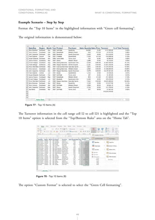
Figure 77 - Top 10 Items (A)
The Turnover information in the cell range cell I2 to cell I21 is highlighted and the “Top
10 Items” option is selected from the “Top/Bottom Rules” area on the “Home Tab”.
Figure 78 - Top 10 Items (B)
The option “Custom Format” is selected to select the “Green Cell formatting”.
CONDITIONAL FORMATTING AND
CONDITIONAL FORMULAS What is Conditional Formatting
50
Figure 79 - Top 10 Items (C)
The “Green Cell formatting” is selected.
Figure 80 - Top 10 Item (D)
The “OK” button for the “Top 10 Items” option is selected to apply the “Green Cell
formatting” to the highlighted Turnover information.
Figure 81 - Top 10 Items (E)
CONDITIONAL FORMATTING AND
CONDITIONAL FORMULAS What is Conditional Formatting
51
The “Green Cell formatting” has now been applied to the Turnover information for the
cell range cell I2 to cell I21.
Figure 82 - Top 10 Items (F)
1.2.2 BOTTOM 10 ITEMS
Information is tested for the Conditional Formatting area “Bottom 10 Items”, when highlighted
spreadsheet information is entered as a numerical entry. The information entered is then
tested using Conditional Formatting, for numerical values for the “Bottom 10 Items” or
tested for other items like the Bottom 4 Items or Bottom 15 Items.
Example Scenario – Step by Step
Format the “Bottom 10 Items” in the Sales Quantity column with “Red cell formatting”.
The original information is demonstrated below:
CONDITIONAL FORMATTING AND
CONDITIONAL FORMULAS What is Conditional Formatting
52
Figure 83 - Bottom 10 Items (A)
The Sales Quantity information in the cell range cell G2 to cell G21 is highlighted and the
“Bottom 10 Items” option is selected from the “Top/Bottom Rules” area on the “Home Tab”.
Figure 84 - Bottom 10 Items (B)
The option “Custom Format” is selected to select the “Red Cell formatting”.
Figure 85 - Bottom 10 Items (C)
CONDITIONAL FORMATTING AND
CONDITIONAL FORMULAS What is Conditional Formatting
53
The “Red Cell formatting” is selected.
Figure 86 - Bottom 10 Items (D)
The “OK” button for the “Bottom 10 Items” option is selected to apply the “Red Cell
formatting” to the highlighted Sales Quantity information.
Figure 87 - Bottom 10 Items (E)
The “Red Cell formatting” has now been applied to the Sales Quantity information for the
cell range cell G2 to cell G21.
CONDITIONAL FORMATTING AND
CONDITIONAL FORMULAS What is Conditional Formatting
54
Figure 88 - Bottom 10 Items (F)
1.2.3 TOP 10 PERCENT
Information is tested for the Conditional Formatting area “Top 10%”, when highlighted
spreadsheet information is entered as a numerical entry. The information entered is then
tested using Conditional Formatting, for numerical values for the “Top 10%” or tested for
other items like the Top 20 percent or Top 30 percent.
Example Scenario – Step by Step
Format the “Top 10%” in the Turnover column with “Green cell formatting”.
The original information is demonstrated below:
CONDITIONAL FORMATTING AND
CONDITIONAL FORMULAS What is Conditional Formatting
55
Figure 89 - Top 10% (A)
The Turnover information in the cell range cell I2 to cell I21 is highlighted and the “Top
10%” option is selected from the “Top/Bottom Rules” area on the “Home Tab”.
Figure 90 - Top 10% (B)
The option “Custom Format” is selected to select the “Green Cell formatting”.
Figure 91 - Top 10% (C)
CONDITIONAL FORMATTING AND
CONDITIONAL FORMULAS What is Conditional Formatting
56
The “Green Cell formatting” is selected.
Figure 92 - Top 10% (D)
The “OK” button for the “Top 10%” option is selected to apply the “Green Cell formatting”
to the highlighted Turnover information.
Figure 93 - Top 10% (E)
The “Green Cell formatting” has now been applied to the Turnover information for the
cell range cell I2 to cell I21.
CONDITIONAL FORMATTING AND
CONDITIONAL FORMULAS What is Conditional Formatting
57
Figure 94 - Top 10% (F)
1.2.4 BOTTOM 10 PERCENT
Information is tested for the Conditional Formatting area “Bottom 10%”, when highlighted
spreadsheet information is entered as a numerical entry. The information entered is then
tested using Conditional Formatting, for numerical values for the “Bottom 10%” or tested
for other items like the Bottom 20 percent or the Bottom 30 percent.
Example Scenario – Step by Step
Format the “Bottom 10%” in the Turnover column with “Red cell formatting”.
The original information is demonstrated below:
Figure 95 - Bottom 10% (A)
CONDITIONAL FORMATTING AND
CONDITIONAL FORMULAS What is Conditional Formatting
58
The Turnover information in the cell range cell I2 to cell I21 is highlighted and the “Bottom
10%” option is selected from the “Top/Bottom Rules” area on the “Home Tab”.
Figure 96 - Bottom 10% (B)
The option “Custom Format” is selected to select the “Red Cell formatting”.
Figure 97 - Bottom 10% (C)
The “Red Cell formatting” is selected.
CONDITIONAL FORMATTING AND
CONDITIONAL FORMULAS What is Conditional Formatting
59
Figure 98 - Bottom 10% (D)
The “OK” button for the “Bottom 10%” option is selected to apply the “Red Cell formatting”
to the highlighted Turnover information.
Figure 99 - Bottom 10% (E)
The “Red Cell formatting” has now been applied to the Turnover information for the cell
range cell I2 to cell I21.
CONDITIONAL FORMATTING AND
CONDITIONAL FORMULAS What is Conditional Formatting
60
Figure 100 - Bottom 10% (F)
1.2.5 ABOVE AVERAGE
Information is tested for the Conditional Formatting area “Above Average”, when highlighted
spreadsheet information is entered as a numerical entry. The information entered is then
tested using Conditional Formatting, for numerical values which are “Above Average” for
selected information.
Example Scenario – Step by Step
Format information which is “Above Average” in the Turnover column with “Green cell
formatting”.
The original information is demonstrated below:
CONDITIONAL FORMATTING AND
CONDITIONAL FORMULAS What is Conditional Formatting
61
Figure 101 - Above Average (A)
The Turnover information in the cell range cell I2 to cell I21 is highlighted and the “Above
Average” option is selected from the “Top/Bottom Rules” area on the “Home Tab”.
Figure 102 - Above Average (B)
The option “Custom Format” is selected to select the “Green Cell formatting”.
Figure 103 - Above Average (C)
CONDITIONAL FORMATTING AND
CONDITIONAL FORMULAS What is Conditional Formatting
62
The “Green Cell formatting” is selected.
Figure 104 - Above Average (D)
The “OK” button for the “Above Average” option is selected to apply the “Green Cell
formatting” to the highlighted Turnover information.
Figure 105 - Above Average (E)
The “Green Cell formatting” has now been applied to the Turnover information for the
cell range cell I2 to cell I21.
CONDITIONAL FORMATTING AND
CONDITIONAL FORMULAS What is Conditional Formatting
63
Figure 106 - Above Average (F)
1.2.6 BELOW AVERAGE
Information is tested for the Conditional Formatting area “Below Average”, when highlighted
spreadsheet information is entered as a numerical entry. The information entered is then
tested using Conditional Formatting, for numerical values which are “Below Average” for
selected information.
Example Scenario – Step by Step
Format information which is “Below Average” in the Turnover column with “Red cell
formatting”.
The original information is demonstrated below:
CONDITIONAL FORMATTING AND
CONDITIONAL FORMULAS What is Conditional Formatting
64
Figure 107 - Below Average (A)
The Turnover information in the cell range cell I2 to cell I21 is highlighted and the “Below
Average” option is selected from the “Top/Bottom Rules” area on the “Home Tab”.
Figure 108 - Below Average (B)
The option “Custom Format” is selected to select the “Red Cell formatting”.
Figure 109 - Below Average (C)
CONDITIONAL FORMATTING AND
CONDITIONAL FORMULAS What is Conditional Formatting
65
The “Red Cell formatting” is selected.
Figure 110 - Below Average (D)
The “OK” button for the “Below Average” option is selected to apply the “Red Cell
formatting” to the highlighted Turnover information.
Figure 111 - Below Average (E)
The “Red Cell formatting” has now been applied to the Turnover information for the cell
range cell I2 to cell I21.
CONDITIONAL FORMATTING AND
CONDITIONAL FORMULAS What is Conditional Formatting
66
Figure 112 - Below Average (F)
1.3 DATA BARS
The use of Data Bars in Conditional Formatting is a very visual use of colour, to display
highlighted spreadsheet information with “coloured bars” according to a specific data criterion,
i.e., apply a green data bar for all sales over £1000. There is a choice of colour settings for
the Data Bars, where standard colour settings or gradient colour settings can be applied to
highlighted spreadsheet information.
Example Scenario – Step by Step
Format the “Turnover Target Review” information with a “Blue Gradient Data Bar” to
compare the selected values, against the “Turnover Target Figure” in cell O1.
The original information is demonstrated below:
CONDITIONAL FORMATTING AND
CONDITIONAL FORMULAS What is Conditional Formatting
67
Figure 113 - Data Bars (A)
The Turnover Target Review information in the cell range cell J2 to cell J21 is highlighted
and the “More Rules” option is selected from the “Data Bars” area on the “Home Tab”.
Figure 114 - Data Bars (B)
The “New Formatting Rule” dialogue box is displayed with the area “Format all cells based
on their values” selected.
CONDITIONAL FORMATTING AND
CONDITIONAL FORMULAS What is Conditional Formatting
68
Figure 115 - Data Bars (C)
The “Minimum” dropdown arrow is selected from the “Type” area, and the “Number”
option is selected from the list of options in this example.
Figure 116 - Data Bars (D)
In the example below the “Minimum Number” has been set to a value of 0 (zero) and the
“Maximum Number” has been set using cell O1 which is the “Target Value” cell (£55000).
The benefit of using cell O1 as the “Maximum Number” is if the “Target Value” is updated
in cell O1, the Data Bar colour will automatically update according to the new target.
CONDITIONAL FORMATTING AND
CONDITIONAL FORMULAS What is Conditional Formatting
69
Figure 117 - Data Bars (E)
The “Gradient Fill” option is now selected from the “Fill” area.
Figure 118 - Data Bars (F)
The “Blue” colour choice is selected from the “Colour” area. The “OK” button is now
selected to apply the Data Bars to the cell range cell J2 to cell J21.
CONDITIONAL FORMATTING AND
CONDITIONAL FORMULAS What is Conditional Formatting
70
Figure 119 - Data Bars (G)
The Blue Data Bars demonstrate the progress of the “Turnover Target Review” information,
against the “Turnover Target” in cell O1 (£55000).
Figure 120 - Data Bars (H)
Data Bars Example Scenario 2 – Step by Step
Format the “Turnover Target Progress” information with a “Blue Gradient Data Bar” against
the “Turnover Target Figure” in cell O1, without displaying the “Turnover Target Progress”
values.
CONDITIONAL FORMATTING AND
CONDITIONAL FORMULAS What is Conditional Formatting
71
The original information is demonstrated below:
Figure 121 - Data Bar No Values (A)
The Turnover Target Progress information in the cell range cell K2 to cell K21 is highlighted
and the “More Rules” option is selected from the “Data Bars” area on the “Home Tab”.
Figure 122 - Data Bar No Values (B)
The “Minimum” dropdown arrow is selected from the “Type” area, and the “Number”
option is selected from the list of options in this example. The option “Show Bar Only”
has also been selected to hide the values in the cell range cell K2 to cell K21 and only
display the Data Bar.
CONDITIONAL FORMATTING AND
CONDITIONAL FORMULAS What is Conditional Formatting
72
Figure 123 - Data Bar No Values (C)
In the example below the “Minimum Number” has been set to a value of 0 (zero) and the
“Maximum Number” has been set using cell O1 which is the “Target Value” cell (£55000).
The benefit of using cell O1 as the “Maximum Number” is if the “Target Value” is updated
in cell O1 the Data Bar colour will automatically update according to the new target.
Figure 124 - Data Bar No Values (D)
The “Gradient Fill” option is now selected from the “Fill” area.
CONDITIONAL FORMATTING AND
CONDITIONAL FORMULAS What is Conditional Formatting
73
Figure 125 - Data Bar No Values (E)
The “Blue” colour choice has now been selected from the “Colour” area. The “OK” button
is now selected to apply the Data Bars to the cell range cell K2 to cell K21.
Figure 126 - Data Bar No Values (F)
Only the Blue Data Bars now demonstrate the progress of the “Turnover Target Progress”
information, against the “Turnover Target” in cell O1 (£55000). In this example if the
values were needed to review the Data Bars in the cell range cell K2 to cell K21, the values
in Column J could be used as these values were duplicated to demonstrate the progress of
the Blue Data Bars, in the cell range cell K2 to cell K21.
CONDITIONAL FORMATTING AND
CONDITIONAL FORMULAS What is Conditional Formatting
74
Figure 127 - Data Bar No Values (G)
Data Bars Example Scenario 3 – Step by Step
Format the positive and negative “Turnover Average Deviation” information in the cell
range cell M2 to cell M21, with “Gradient Fill” Data Bars.
The original information is demonstrated below:
Figure 128 - Data Bar Negative Values (A)
The Turnover Average Deviation information in the cell range cell M2 to cell M21 is
highlighted and the “More Rules” option is selected from the “Data Bars” area on the
“Home Tab”.
CONDITIONAL FORMATTING AND
CONDITIONAL FORMULAS What is Conditional Formatting
75
Figure 129 - Data Bar Negative Values (B)
The option “Show Bar Only” is selected, and the positive values is selected as a Blue
Gradient colour. The “Negative Value and Axis” option is now selected to set the negative
values option.
Figure 130 - Data Bar Negative Values (C)
The “Negative Bar Fill Colour” is set as a “Red” Fill and the Axis Settings area is selected
with the “Cell Midpoint” option. The “OK” button is now selected to set the “Negative
Value and Axis Settings”.
CONDITIONAL FORMATTING AND
CONDITIONAL FORMULAS What is Conditional Formatting
76
Figure 131 - Data Bar Negative Values (D)
The “OK” button is now selected to apply the positive and negative Data Bar settings.
Figure 132 - Data Bar Negative Values (E)
The positive and negative Data Bar settings are displayed for the cell range cell M2 to cell M21.
Figure 133 - Data Bar Negative Values (F)
CONDITIONAL FORMATTING AND
CONDITIONAL FORMULAS What is Conditional Formatting
77
1.4 COLOUR SCALES
The use of Colour Scales in Conditional Formatting is a very visual use of colour, to display
highlighted spreadsheet information with “coloured cells” which vary in colour according
to a specific data criterion, i.e., apply a green shading for all sales over £1000.
Example Scenario – Step by Step
Format the “Turnover” information with red cell formatting for the low value of 1000,
Orange cell formatting for the midpoint value of 20000 and Yellow cell formatting for the
high value of 55000 (Turnover Target – cell O1).
The original information is demonstrated below:
Figure 134 - Colour Scales (A)
The Turnover Information in the cell range cell I2 to cell I21 is highlighted and the “More
Rules” option is selected from the “Colour Scales” area on the “Home Tab”.
Figure 135 - Colour Scales (B)
CONDITIONAL FORMATTING AND
CONDITIONAL FORMULAS What is Conditional Formatting
78
The “Format Style” dropdown arrow is selected, and the “3-Colour Scale” option is selected
from the list of options in this example.
Figure 136 - Colour Scales (C)
The “Minimum” dropdown arrow is selected from the “Type” area, and the “Number”
option is selected from the list of options in this example.
Figure 137 - Colour Scales (D)
In the example below the “Minimum Number” has been set to a value of 1000, the
“Midpoint Number” has been set to 20000 and the “Maximum Number” has been set to
55000, which is the Target Value (Cell O1). The Yellow Colour applied for the Maximum
Value is applied to any value which is 55000 or more.
CONDITIONAL FORMATTING AND
CONDITIONAL FORMULAS What is Conditional Formatting
79
Figure 138 - Colour Scales (E)
The colour scales applied to the cell range cell I2 to cell I21, demonstrate the progress of the
“Turnover” information, against the “Turnover Target” in cell O1 (£55000). Any “Turnover”
information which has reached the “Turnover Target” of 55000 has yellow shading applied
to the cell value. Any values which have not reached 55000, are coloured in shades of Red
and Orange and the shading appears a lighter shade of orange, the closer the Turnover value
is to the “Turnover Target” of 55000.
Figure 139 - Colour Scales (F)
Colour Scales Example 2 Scenario – Step by Step
Format the “Monthly Turnover” information with red, orange and yellow cell formatting
with Red cell formatting applied for the low value of 500, Orange cell formatting for the
midpoint value of 3000 and Yellow cell formatting for the high value of 7000.
CONDITIONAL FORMATTING AND
CONDITIONAL FORMULAS What is Conditional Formatting
80
The original information is demonstrated below with all the monthly turnover values hidden
to apply colour shading to the cell range cell B5 to cell M9:
Figure 140 - Colour Scales Heat Map (A)
The hidden figures are demonstrated below where monthly turnover values range from
£600 to £6700.
Figure 141 - Colour Scales Heat Map (B)
The Turnover Information in the cell range cell B5 to cell M9 is highlighted and the “More
Rules” option is selected from the “Colour Scales” area on the “Home Tab”.
Figure 142 - Colour Scales Heat Map (C)
CONDITIONAL FORMATTING AND
CONDITIONAL FORMULAS What is Conditional Formatting
81
In the example below the “Minimum Number” has been set to a value of 1000, the “Midpoint
Number” has been set to 3000 and the “Maximum Number” has been set to 7000.
Figure 143 - Colour Scales Heat Map (D)
The “Heat Map” demonstrates where the high, low and midpoint turnover values are,
through the use of colour only with no values displayed.
Figure 144 - Colour Scales Heat Map (E)
1.5 ICON SETS
The use of Icon Set in Conditional Formatting is a very visual use of coloured Images, to
display highlighted spreadsheet information with a certain coloured Icon Image according
to specified data criterion, i.e., add a green arrow to all cells with sales over £1000.
CONDITIONAL FORMATTING AND
CONDITIONAL FORMULAS What is Conditional Formatting
82
Example Scenario – Step by Step
Format all Turnover cells in the cell range I2 to cell I21 which have a turnover value between
5000 and 20000, with a “Yellow Ball Icon”.
The original information is demonstrated below:
Figure 145 - Icon Sets (A)
The Turnover Information in the cell range cell I2 to cell I21 is highlighted and the “More
Rules” option is selected from the “Icon Sets” area on the “Home Tab”.
Figure 146 - Icon Sets (B)
Under the “Type” area the “Number” option is selected, in this example.
CONDITIONAL FORMATTING AND
CONDITIONAL FORMULAS What is Conditional Formatting
83
Figure 147 - Icon Sets (C)
When completing the values area for the different coloured “Icons”, the highest value of
20000 is entered first and a “Green Icon” is applied for any turnover value which is greater
than () 20000. With the first test reviewing information greater than 20000, the second test
now reviews all turnover values which are less than or equal to (=) 20000 and a “Yellow
Icon” is applied if this criterion is met. The final test reviews turnover values which are less
than () 5000 and a “Red Icon” is applied if this criterion is met. The “Green and Red
Icons” will be removed, as only the “Yellow” Icon is required.
Figure 148 - Icon Sets (D)
The “Green Icon” is now removed by selecting the option “No Cell Icon”. The “Red Icon”
will also be removed by selecting the “No Cell Icon” option.
CONDITIONAL FORMATTING AND
CONDITIONAL FORMULAS What is Conditional Formatting
84
Figure 149 - Icon Sets (E)
With only the “Yellow Icon” now visible the “OK” button is selected. Only the “Yellow
Icon” will now be displayed for all Turnover values between 5000 and 20000 (inclusive).
Figure 150 - Icon Sets (F)
The “Yellow Icon” has now been applied to all Turnover values between 5000 and 20000.
CONDITIONAL FORMATTING AND
CONDITIONAL FORMULAS What is Conditional Formatting
85
Figure 151 - Icon Sets (G)
Example Scenario Positive and Negative Values – Step by Step
Display “Green and Red Icon Sets” only for all “Average Deviation Status” positive and
negative values, in the cell range cell N2 to cell N21.
The original information is demonstrated below:
Figure 152 - Icon Sets Positive/Negative Values (A)
The Average Deviation Status Information in the cell range cell N2 to cell N21 is highlighted
and the “More Rules” option is selected from the “Icon Sets” area on the “Home Tab”.
CONDITIONAL FORMATTING AND
CONDITIONAL FORMULAS What is Conditional Formatting
86
Figure 153 - Icon Sets Positive/Negative Values (B)
The “Icon Set” has been setup in the example below, where the “Green Arrow” has been
selected for positive values and the “Red Arrow” has been selected for negative values. The
“Show Icon Only” option is selected and the “OK” button is selected to apply the arrows
for the positive and negative values.
Figure 154 - Icon Sets Positive/Negative Values (C)
The “Green and Red Arrow Icons” are displayed for the “Average Deviation Status” values.
CONDITIONAL FORMATTING AND
CONDITIONAL FORMULAS What is Conditional Formatting
87
Figure 155 - Icon Sets Positive/Negative Values (D)
1.6 NEW RULE
The New Rule option is another way of using conditional formatting features like “Highlight
Cell Rules”, “Top 10 Items” etc. The New Rule option is a conditional formatting option
and is available on the Home Tab and is demonstrated below.
Figure 156 - New Rule (A)
The “New Formatting Rule” box is demonstrated below with multiple options available
including “Above or Below Average”. The only area which is only available through the
“New Rule” option, is “Use a formula to determine which cells to format”. This area will
now be selected to apply a formula to selected information.
CONDITIONAL FORMATTING AND
CONDITIONAL FORMULAS What is Conditional Formatting
88
Figure 157 - New Rule (B)
An example of a formula created in the “Use a formula to determine which cells to format”
area is demonstrated below.
Figure 158 - New Rule (C)
1.7 MANAGE RULES AND EDITING RULES
The Manage Rule option is used to modify and make changes to conditional formatting
settings. The option Manage Rules is available from the conditional formatting options on
the Home Tab.
CONDITIONAL FORMATTING AND
CONDITIONAL FORMULAS What is Conditional Formatting
89
Figure 159 - Manage Rules (A)
The “Bottom 3” rule is selected and is to be modified and updated to the “Bottom 6”. The
“Edit Rule” button is selected to modify the selected rule.
Figure 160 - Manage Rules (B)
The bottom 3 is updated to the bottom 6 and the “OK” button is selected.
CONDITIONAL FORMATTING AND
CONDITIONAL FORMULAS What is Conditional Formatting
90
Figure 161 - Manage Rules (C)
The selected rule has been updated to the “Bottom 6” and the “Applies to” area demonstrates
the cell range the rule is applied to, in this example cell I2 to cell I21. This range can also
be modified if required. The “OK” button is now selected to update the rule.
Figure 162 - Manage Rules (D)
The “Bottom 3” which is formatted with red cell formatting, is updated to the “Bottom 6”.
CONDITIONAL FORMATTING AND
CONDITIONAL FORMULAS What is Conditional Formatting
91
Figure 163 - Manage Rules (E)
1.8 CLEARING CONDITIONAL FORMATTING
Conditional Formatting rules are to be removed from the selected information cell I2 to cell
I21. This is achieved by selecting the “Clear Rules” option from the conditional formatting
area, then in this example selecting the “Clear Rules from Selected Cells” option.
Figure 164 - Clearing Rules (A)
The conditional formatting rules have now been removed from the cell range cell I2 to
cell I21.
CONDITIONAL FORMATTING AND
CONDITIONAL FORMULAS What is Conditional Formatting
92
Figure 165 - Clearing Rules (B)
1.9	
MULTIPLE CONDITIONAL FORMATTING
EXAMPLE (HIGHLIGHT CELL RULES)
The example scenario is displayed below.
Figure 166 - Multiple Conditional Formatting (A)
The scenario information is demonstrated below, and conditional formatting will be added
to the cell range cell J2 to cell J21.
CONDITIONAL FORMATTING AND
CONDITIONAL FORMULAS What is Conditional Formatting
93
Figure 167 - Multiple Conditional Formatting (B)
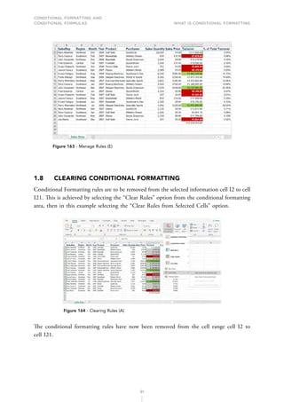
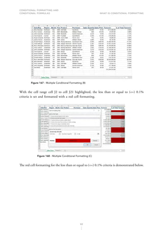
With the cell range cell J2 to cell J21 highlighted, the less than or equal to (=) 0.1%
criteria is set and formatted with a red cell formatting.
Figure 168 - Multiple Conditional Formatting (C)
The red cell formatting for the less than or equal to (=) 0.1% criteria is demonstrated below.
CONDITIONAL FORMATTING AND
CONDITIONAL FORMULAS What is Conditional Formatting
94
Figure 169 - Multiple Conditional Formatting (D)
With the cell range cell J2 to cell J21 highlighted, the less than or equal to (=) 1% criteria
is set and formatted with a green cell formatting.
Figure 170 - Multiple Conditional Formatting (E)
Since there are now two “less than or equal to” scenarios set, this can cause a conflict
between the two scenarios. To avoid this conflict the “Stop If True” option is selected for
the red conditional formatting, so this conditional formatting rule is protected to avoid any
conflict. The “Stop If True” option is very important when multiple conditional formatting
criteria are used, to stop criteria conflict issues and incorrect information colour shading.
CONDITIONAL FORMATTING AND
CONDITIONAL FORMULAS What is Conditional Formatting
95
Figure 171 - Multiple Conditional Formatting (F)
With the cell range cell J2 to cell J21 highlighted, the greater than or equal to (=) 14%
criteria is set and formatted with a different green cell formatting.
Figure 172 - Multiple Conditional Formatting (G)
All the different rules are demonstrated below.
CONDITIONAL FORMATTING AND
CONDITIONAL FORMULAS What is Conditional Formatting
96
Figure 173 - Multiple Conditional Formatting (H)
The information for the cell range cell J2 to cell J21 is shaded according to the three different
conditional formatting scenarios.
Figure 174 - Multiple Conditional Formatting (I)
CONDITIONAL FORMATTING AND
CONDITIONAL FORMULAS Conditional Formatting Formulas
97
2	CONDITIONAL FORMATTING
FORMULAS
There are many ways of applying conditional formatting to highlighted information, so
colour is applied to certain spreadsheet information. A very powerful way of applying colour
to selected spreadsheet information, is to use conditional formatting formulas. The ability
to create formulas is very important when using a spreadsheet and this is very much the
case to get the best out of conditional formatting, through the use of formulas.
To apply a conditional formatting formula to highlighted spreadsheet information the
conditional formatting option “New Rule” is required, and this option is demonstrated below.
Figure 175 - New Formatting Rule_ Using Formulas
2.1	
CREATING CONDITIONAL FORMULAS
AND CELL REFERENCING
The ability to create formulas and use functions is very important when developing advanced
skills in the use of conditional formatting. This book covers the use of formulas and functions
in conditional formatting, but the book does not cover creating formulas. There are other
books I have created which cover how to create formulas and complex formulas and these
books can be purchased by anyone wanting to develop their skills in creating formulas.
CONDITIONAL FORMATTING AND
CONDITIONAL FORMULAS Conditional Formatting Formulas
98
A fundamental part of creating formulas is the use of cell referencing ($ signs) techniques,
to ensure certain parts of a formula are fixed in place when copying a formula within a
spreadsheet. The use and control of cell referencing is essential to creating conditional
formatting formulas and the different cell referencing options will now be discussed and
demonstrated.
Absolute Cell Refencing (Fixing a cell)
This form of cell referencing adds two-dollar signs ($) to a part of a formula, to fix a part
of a formula in place. This method of cell referencing is demonstrated below.
A formula has been created in cell F5 and the formula is demonstrated in the formula
bar. The formula will be copied down Column F and the formula will be incorrect when
copied, as the H3 part of the formula will move. For the formula to be correct when it is
copied down Column F, the H3 part of the formula must not move so each formula can
be increased by the 10% increase in cell H3.
Figure 176 - Absolute Cell Referencing (A)
The example below demonstrates when the formula is copied down Column F, the formula
is incorrect as the formulas do not increase by 10%. The formula in cell F6 demonstrates
this with the formula displaying the value of £3300, where the correct answer with a 10%
increase should read £36300.
CONDITIONAL FORMATTING AND
CONDITIONAL FORMULAS Conditional Formatting Formulas
99
Figure 177 - Absolute Cell Referencing (B)
In the example below the formula in cell F5 is corrected where dollar signs ($) are added
to the formula to correct the formula and the formula is then copied down Column F.
The formula is now correct when it is copied down Column F and all the formulas have
increased by 10%.
Figure 178 - Absolute Cell Referencing (C)
Relative Cell Refencing (Fixing part of a cell)
This form of cell referencing adds one dollar sign ($) to a part(s) of a formula, to fix a
part(s) of a formula in place. This method of cell referencing is demonstrated below. A
formula has been created in cell G4 and the formula is demonstrated in the formula bar.
The formula in cell G4 will be copied to cell L23 to increase all the salaries in Column E
by all the percentages in row 3. In this example the formula in cell G4 is to be copied down
CONDITIONAL FORMATTING AND
CONDITIONAL FORMULAS Conditional Formatting Formulas
100
Column G and across row 4. When the formula is copied to cell L23 the answer in cell
L23 must be the same as the £105,000 in cell M23 which is a 50% increase of the salary
in cell E23. The formula in cell G4 will now be copied to cell H4 and cell G5 without the
use of cell referencing and the answers in these cells will be incorrect.
Figure 179 - Relative Cell Referencing (A)
The formulas in cell G5 and H4 are incorrect. Cell G5 should display the salary in cell E5
increased by 25% and cell H4 should display the salary in cell E4 increased by the 30%
in cell H3. When the formula in cell G4 is copied to cell G5 the G3 part of the formula
changes to G4 and the formula moves away from the 25% in cell G3. When the formula
is copied to cell H4 the E4 part of the formula moves away from the £35,000 in cell E4.
In this formula, to correct the formula in cell G4 both parts of the formula E4 and G3
must be “fixed”, using cell referencing techniques.
Figure 180 - Relative Cell Referencing (B)
The formula in cell G4 has now been corrected using relative cell referencing techniques,
where the E is fixed for the E4 part of the formula and the 3 is fixed for the G3 part of the
formula. The formula in cell G4 has been copied correctly to cell L23 and the value displayed
in cell L23 is £105,000, this value represents a 50% increase of the salary in cell E23.
CONDITIONAL FORMATTING AND
CONDITIONAL FORMULAS Conditional Formatting Formulas
101
Figure 181 - Relative Cell Referencing (C)
I have produced MS Excel books and online videos which are available for a more detailed
explanation of cell referencing techniques in formulas and functions.
2.2	
CONDITIONAL FORMULA SIGNS AND
USING SIGNS IN FORMULAS
When creating conditional formatting formulas there is often a need to use criteria signs
when constructing the formula. The main criteria signs used in conditional formatting
formulas are demonstrated below.
Figure 182 - Criteria Signs (A)
An example of a formula where criteria signs are used is demonstrated below in cell I8. The
formula demonstrated with criteria signs is used to apply the green cell formatting for the
spreadsheet information starting in cell A3.
CONDITIONAL FORMATTING AND
CONDITIONAL FORMULAS Conditional Formatting Formulas
102
Figure 183 - Criteria Signs (B)
2.3 APPLYING FORMULA FORMATTING
When a conditional formatting formula has been created and the formula formatting has
been applied to a single cell or range of cells, there may be a need to copy the formula
formatting to other cells in a spreadsheet. There are two main methods to copy conditional
formatting formulas, namely, “Format Painter” and “Paste Special”. These two methods with
now be demonstrated.
2.3.1 FORMAT PAINTER
In the example below the Average function has been used to create a conditional formatting
formula and the formatting for the formula has been applied to cell B6. The formatting
for the conditional formatting formula will now be applied to the cell range cell B7 to cell
B19, using the “Format Painter”.
Figure 184 - Format Painter (A)
CONDITIONAL FORMATTING AND
CONDITIONAL FORMULAS Conditional Formatting Formulas
103
In the example below cell B6 has been selected and the Format Painter feature which is
located on the Home tab is used to copy the conditional formatting formula format in
cell B6.
Figure 185 - Format Painter (B)
The cell range cell B7 to cell B19 has now been highlighted with the Format Painter feature
to copy the formatting and the conditional formatting formula format has been applied to
the cell range cell B7 to cell B19.
Figure 186 - Format Painter (C)
2.3.2 PASTE SPECIAL
In the example below the Average function has been used to create a conditional formatting
formula and the formatting for the formula has been applied to cell B6. The formatting
for the conditional formatting formula will now be applied to the cell range cell B7 to cell
B19, using the “Paste Special” feature.
CONDITIONAL FORMATTING AND
CONDITIONAL FORMULAS Conditional Formatting Formulas
104
Figure 187 - Paste Special (A)
Cell B6 which has the conditional formatting formula is copied and the cell range cell B7
to cell B19 is selected.
Figure 188 - Paste Special (B)
The “Paste Special” feature is now selected from the Home Tab.
Figure 189 - Paste Special (C)
CONDITIONAL FORMATTING AND
CONDITIONAL FORMULAS Conditional Formatting Formulas
105
The Paste Special option “Formats” is selected and the “OK” button is selected to apply the
conditional formatting formula in cell B6, to the cell range cell B7 to cell B19.
Figure 190 - Paste Special (D)
The formula formatting in cell B6 has been applied to the cell range cell B7 to cell B19.
Figure 191 - Paste Special (E)
2.4 TESTING CONDITIONAL FORMATTING FORMULAS
When creating conditional formatting formulas, it can be difficult at times to write a formula
in the formula area of the New Rule box, which is demonstrated below. There is a need
to check the result of conditional formatting formulas to test for “True” and “False” result
outputs from any detailed formula. If a conditional formatting formula produces a “True”
or “False” result the formula can be used to add formatting to a range of highlighted cells.
The New Rule box demonstrated below is acceptable for producing simple formulas which
CONDITIONAL FORMATTING AND
CONDITIONAL FORMULAS Conditional Formatting Formulas
106
can be checked easily for “correctness”, but not for more complex conditional formatting
formulas which are very detailed. Testing conditional formatting formulas for “True” and
“False” output results will now be reviewed.
Figure 192 - Testing Conditional Formatting Formulas (A)
2.4.1 TESTING FOR “TRUE” AND “FALSE” FORMULA RESULTS
The example below demonstrates a “True” or “False” testing area for formulas which have
produced a “True” or “False” formula result. The “True” or “False” formula results in the
cell range cell I5 to cell I8 have been created for the colours “White”, “Yellow”, “Red” and
“Green” in the cell range cell H5 to cell H8. The “True” or “False” formula results in the
testing area have been copied to the “Conditional Formatting Formulas” area and applied
to the cell range cell A2 to cell E13. This is an example where formulas tested successfully
for “True” or “False” results, can be copied to produce effective conditional formatting
results. The “True” and “False” formula results in the cell range cell I5 to cell I8, will now
be reviewed to demonstrate the effectiveness of producing formulas with “True” or “False”
results for conditional formatting formula purposes.
Figure 193 - True or False Testing (A)
CONDITIONAL FORMATTING AND
CONDITIONAL FORMULAS Conditional Formatting Formulas
107
The “False” result formula for cell I8 is demonstrated below. The formula tests whether
cell B2 equals “IT Skills” and cell E2 is greater than or equal to (=) 5 OR whether cell
B2 equals “Business Skills” and cell E2 is greater than or equal to (=) 5. If either of these
conditions are met then a “True” result is returned, if this is not the case a “False” result
is returned. The result for the test cell I8 returns a “False” result as neither of the tested
conditions are met for the tests undertaken for cell B2 or cell E2. When the test result in
cell I8 was copied as a conditional formatting formula to the cell range cell A2 to cell E13,
the tested formula produced multiple “Green” cell results, as demonstrated in the example
above. The same process was followed to copy the “True” results in the cell range cell I5 to
cell I7 and in applying the test results to the cell range cell A2 to cell E13.
Figure 194 - True or False Testing (B)
2.4.2 COPYING AND PASTING TESTED FORMULAS
The tested formula in cell I8 which displays a “False” formula result will now be copied to
the conditional formatting formula area. Any formula test result which displays a “True”
or “False” result can be copied as a conditional formatting formula.
Figure 195 - Copying a Tested Formula (A)
CONDITIONAL FORMATTING AND
CONDITIONAL FORMULAS Conditional Formatting Formulas
108
It is easier to copy a tested formula by adding an inverted comma(‘) at the start of the formula
in the formula bar, which then displays the formula in the selected cell as demonstrated
below.
Figure 196 - Copying a Tested Formula (B)
The formula is now selected in the formula bar, except the inverted comma (‘) and the copy
option is selected to copy the formula in the formula bar.
Figure 197 - Copying a Tested Formula (C)
After copying the formula, the cell range cell A2 to cell E12 is selected to apply the
conditional formatting as demonstrated below. The conditional formatting option “New
Rule” is now selected to add the conditional formula formatting.
CONDITIONAL FORMATTING AND
CONDITIONAL FORMULAS Conditional Formatting Formulas
109
Figure 198 - Copying a Tested Formula (D)
The option “Use a formula to determine which cell to format” is selected.
Figure 199 - Copying a Tested Formula (E)
The formula has now been copied to this area using the “Paste” option. The format button
option is now selected to add the cell colouring for the formula, which in this example is
green cell formatting.
CONDITIONAL FORMATTING AND
CONDITIONAL FORMULAS Conditional Formatting Formulas
110
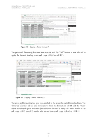
Figure 200 - Copying a Tested Formula (F)
The green cell formatting has now been selected and the “OK” button is now selected to
apply the formula shading to the cell range cell A2 to cell E13.
Figure 201 - Copying a Tested Formula (G)
The green cell formatting has now been applied to the areas the copied formula affects. The
“Inverted Comma” (‘) has also been remove from the formula in cell I8 and the “False”
result is displayed again. The same process would be used to apply the “True” results in the
cell range cell I5 to cell I7 to the information in the cell range cell A2 to cell E12.
CONDITIONAL FORMATTING AND
CONDITIONAL FORMULAS Conditional Formatting Formulas
111
Figure 202 - Copying a Tested Formula (H)
2.5	
CONTROLLING AND ORDERING FORMULA
FORMATTING (“STOP IF TRUE”)
When multiple conditional formatting formula rules are applied to selected information,
like the example demonstrated below, there may be a requirement to change the order of
the rules by reordering the rules. With multiple rules there could also be a requirement to
use the “Stop If True” feature, to ensure there is no conflict between rules. The “Ordering”
and “Stop If True” features will now be demonstrated to manage multiple conditional
formatting rules.
Figure 203 - Controlling and Ordering Formatting (A)
In the example below the cell range cell A2 to cell E13 is highlighted and the “Manage
Rules” option is selected from the Conditional Formatting area. The “Manage Rules” option
is used to modify conditional formatting rules, change the order of rules, and use the “Stop
If True” option.
CONDITIONAL FORMATTING AND
CONDITIONAL FORMULAS Conditional Formatting Formulas
112
Figure 204 - Controlling and Ordering Formatting (B)
The rules applied to the cell range cell A2 to cell E13 is demonstrated below. The rules have
been created for “White”, “Yellow”, “Red” and “Green” shading. The rules for the different
colour shading will now be reviewed.
Figure 205 - Controlling and Ordering Formatting (C)
The “White Shading” rule, which is displayed below, tests cell B2 to check if the cell contains
either “IT Skills” or “Business Skills” and whether cell E2 is blank.
CONDITIONAL FORMATTING AND
CONDITIONAL FORMULAS Conditional Formatting Formulas
113
Figure 206 - Controlling and Ordering Formatting (D)
The “Yellow Shading” rule, which is displayed below, tests cell B2 to check if the cell
contains either “IT Skills” or “Business Skills” and whether cell E2 has no delegate numbers
entered (0).
Figure 207 - Controlling and Ordering Formatting (E)
The “Red Shading” rule, which is displayed below, tests cell B2 to check if the cell contains
“IT Skills” and if cell E2 is less than 5 delegates or if cell B2 contains “Business Skills” and
if cell E2 is less than 5 delegates.
CONDITIONAL FORMATTING AND
CONDITIONAL FORMULAS Conditional Formatting Formulas
114
Figure 208 - Controlling and Ordering Formatting (F)
The “Green Shading” rule, which is displayed below, tests cell B2 to check if the cell contains
“IT Skills” and if cell E2 is greater than or equal to 5 delegates or if cell B2 contains
“Business Skills” and if cell E2 is greater than or equal to 5 delegates.
Figure 209 - Controlling and Ordering Formatting (G)
In the example below the “Red Shading” rule is selected to demonstrate reordering rules.
A rule could be reordered if required by selecting the “Move Up” of “Move Down” arrow.
In this example the “Move Up” arrow is demonstrated for re-ordering purposes.
CONDITIONAL FORMATTING AND
CONDITIONAL FORMULAS Conditional Formatting Formulas
115
Figure 210 - Controlling and Ordering Formatting (H)
In the example below the “White Shading” rule is selected where the option “Stop If True”
is selected and this option will now be demonstrated. The option “Stop If True” has been
selected for this rule due to cell E2 being tested to see if the cell is blank and the “Yellow
Shading” rule also tests cell E2 for zero (0) delegates. Both tests on cell E2 for both shading
rules would cause a “test conflict” if the “Stop If True” option is not used for the “White
Shading” rule.
Figure 211 - Controlling and Ordering Formatting (I)
2.6 MANAGING AND EDITING FORMULA RESULTS
The information below demonstrates “Green” and “Red” shading applied to cells in the
cell range cell C4 to cell F7. The “Green Shading” has been applied where there is a 10%
increase against the “Average Target” using the “Average Target” figures from cell B12 to
cell B15. The “Red Shading” is applied where there is a 10% decrease against the “Average
Target” using the “Average Target” figures from cell B12 to cell B15.
CONDITIONAL FORMATTING AND
CONDITIONAL FORMULAS Conditional Formatting Formulas
116
Figure 212 - Managing Formula Formatting (A)
The “Green Shading” rule will now be modified to shade cells green, only if there is a 20%
increase against the “Average Target” using the “Average Target” figures from cell B12 to
cell B15.
Figure 213 - Managing Formula Formatting (B)
With the cell range cell C4 to cell F7 selected the “Manage Rules” option is used to update
the “Green Shading” rule.
CONDITIONAL FORMATTING AND
CONDITIONAL FORMULAS Conditional Formatting Formulas
117
Figure 214 - Managing Formula Formatting (C)
The “Green Shading” rule has been selected and the “Edit Rule” button is selected to edit
the rule.
Figure 215 - Managing Formula Formatting (D)
The 10% increase part of the formula has been selected and will be updated.
CONDITIONAL FORMATTING AND
CONDITIONAL FORMULAS Conditional Formatting Formulas
118
Figure 216 - Managing Formula Formatting (E)
The formula has now been updated to increase the rule by 20%. The “OK” button is now
selected to update the rule.
Figure 217 - Managing Formula Formatting (F)
With the “Green Shading” rule selected the “Apply” button is selected to review the “Green
Shading” update.
CONDITIONAL FORMATTING AND
CONDITIONAL FORMULAS Conditional Formatting Formulas
119
Figure 218 - Managing Formula Formatting (G)
The benefit of using the “Apply” button is the rule can be updated quickly if the rule is
incorrect. In this example the “Green Shading” rule is correct and the “OK” button is
selected to complete the rule update.
Figure 219 - Managing Formula Formatting (H)
The updated “Green Shading” has been applied to the cell range cell C4 to cell F7.
CONDITIONAL FORMATTING AND
CONDITIONAL FORMULAS Conditional Formatting Formulas
120
Figure 220 - Managing Formula Formatting (I)
2.7 HIDING “ZERO” VALUES AND/OR PERCENTAGES
In the example below an MS Excel “Pivot Table” is demonstrated and percentages (%)
values are displayed. All the percentages which are equal to 0%, will be hidden so only
percentages which are greater than 0% will be displayed.
Figure 221 - Hiding Zero Values (A)
All the percentage information is highlighted, and the “New Rule” option is selected.
CONDITIONAL FORMATTING AND
CONDITIONAL FORMULAS Conditional Formatting Formulas
121
Figure 222 - Hiding Zero Values (B)
In the formula area cell B3 is tested to check if the cell is greater than zero (0). The
formatting has been selected as “White Font” formatting.
Figure 223 - Hiding Zero Values (C)
All the zero percentage (0%) values have now been hidden, which makes the information
easier to interpret.
CONDITIONAL FORMATTING AND
CONDITIONAL FORMULAS Conditional Formatting Formulas
122
Figure 224 - Hiding Zero Values (D)
2.8 CONDITIONAL FORMATTING FORMULA EXAMPLES
The use of formulas in conditional formatting is an extremely powerful area in MS Excel
and several examples will now be demonstrated. The formula examples will only provide
demonstrations of what can be achieved with the use of formulas in conditional formatting
and the demonstrations will not be covered in great detail. There is a requirement to be
good at using and creating formulas in MS Excel, to be able to use conditional formatting
formulas to a good level.
If anyone needs support or assistance in creating formulas, using functions, and creating
conditional formatting formulas, I have produced books and videos on creating formulas,
using functions, and creating conditional formatting formulas. These products can be
previewed and purchased by visiting the NILC Training website (www.nilc.co.uk).
2.8.1 TARGET SETTING FORMULAS
Example 1
The example below uses formulas to manage targets using colour settings. The quarterly
information displayed in the cell range cell C4 to cell F7, is analysed against the targets
set in the cell range cell B12 to cell B15 for each of the different regions. The quarterly
information will display “Green” cell shading if there the quarterly figures are 10% greater
than the quarterly target and “Red” shading if the quarterly figures are 10% less than the
quarterly target.
CONDITIONAL FORMATTING AND
CONDITIONAL FORMULAS Conditional Formatting Formulas
123
Figure 225 - Target Setting Formulas (A)
The cell range cell C4 to cell F4 is selected. The green shading formula (=C4$B12*1.1)
and red shading formula (=C4$B12*0.90) have been applied to the selected cell range.
Figure 226 - Target Setting Formulas (B)
The quarterly figures with a 10% increase are displayed in “Green shading” and the figures
with a 10% decrease are displayed in “Red” shading. Quarterly figures which do not meet
either criterion have no shading applied.
CONDITIONAL FORMATTING AND
CONDITIONAL FORMULAS Conditional Formatting Formulas
124
Figure 227 - Target Setting Formulas (C)
Example 2
The example below uses formulas to manage monthly turnover changes using colour settings.
The cell range cell B16 to cell M6 is analysed to compare monthly turnover figures with
the previous monthly turnover figure. Formulas are used to compare the monthly turnover
figures and “Green Shading” is applied if the month selected is greater than the previous
month. If this is not the case and the month selected is less than the previous month, then
“Red Shading” is applied.
Figure 228 - Target Setting Formulas (D)
The cell range cell C16 to cell M16 is selected and the formulas are demonstrated below
for the “Green Shading” (=C16B16) and “Red Shading” (=C16B16).
CONDITIONAL FORMATTING AND
CONDITIONAL FORMULAS Conditional Formatting Formulas
125
Figure 229 - Target Setting Formulas (E)
The completed example with shading applied is demonstrated below.
Figure 230 - Target Setting Formulas (F)
2.8.2 DATE CONTROL FORMULAS
The example below uses formulas to manage dates in the cell range cell B3 to cell E7 using
colour settings and the dates are compared to the date displayed in cell H1, which uses the
“Today” function. The Key for the colour settings is demonstrated below and formulas have
been tested for the different colour settings in the cell range cell A11 to cell A14.
CONDITIONAL FORMATTING AND
CONDITIONAL FORMULAS Conditional Formatting Formulas
126
Figure 231 - Date Control Formulas (A)
All the colours have been applied to the cell range cell B3 to cell E7, following the colour
“Key” conditions. The formula for the “Orange Shading” is demonstrated in cell A12.
Figure 232 - Date Control Formulas (B)
All the colour formulas which have been used to apply the colour settings to the cell range
cell B3 to cell E7, are demonstrated below.
Figure 233 - Date Control Formulas (C)
CONDITIONAL FORMATTING AND
CONDITIONAL FORMULAS Conditional Formatting Formulas
127
The completed example is demonstrated below with the colour settings applied to the cell
range cell B3 to cell E7.
Figure 234 - Date Control Formulas (D)
2.8.3 HIGHLIGHTING DUPLICATE ROWS (COUNTIFS FUNCTION)
The example below is used to demonstrate highlighting duplicate information using the
“Countifs” function. The test area from cell L1 to cell M7 is used to test how many “Countifs”
functions are required to apply colour settings to duplicate information. Duplicate values
are demonstrated below where values in row 4 and row 23 are highlighted. These values
plus any other duplicate values will be highlighted using colour settings.
Figure 235 - Duplicate Rows Countifs (A)
In this example 3 “Countifs” are required, and the 3 ranges are tested to check for duplicates
(1). The “Countifs” formula is demonstrated in cell L5.
CONDITIONAL FORMATTING AND
CONDITIONAL FORMULAS Conditional Formatting Formulas
128
Figure 236 - Duplicate Rows Countifs (B)
The formula rule has now been created and applied with 3 “Countifs” functions used. The
rule has “Red Shading” applied to any duplicate values.
Figure 237 - Duplicate Rows Countifs (C)
The completed example is demonstrated below.
Figure 238 - Duplicate Rows Countifs (D)
CONDITIONAL FORMATTING AND
CONDITIONAL FORMULAS Conditional Formatting Formulas
129
2.8.4 HIGHLIGHTING ENTIRE ROWS WITH FORMULAS
Example 1
The information demonstrated below will be used to highlight rows of information according
to a set scenario.
Figure 239 - Highlighting Entire Rows (A)
The scenario for highlighting multiple rows of information in this example is demonstrated
below.
Figure 240 - Highlighting Entire Rows (B)
The scenario formatting is demonstrated below. The formula formatting required a formula
that combined the “SumIfs” and “CountIf” functions.
CONDITIONAL FORMATTING AND
CONDITIONAL FORMULAS Conditional Formatting Formulas
130
Figure 241 - Highlighting Entire Rows (C)
The highlighted rows are demonstrated below according to the set scenario. The completed
formula is demonstrated below the highlighted information.
Figure 242 - Highlighting Entire Rows (D)
Example 2
The information demonstrated below will be used to highlight rows of information according
to a set scenario.
CONDITIONAL FORMATTING AND
CONDITIONAL FORMULAS Conditional Formatting Formulas
131
Figure 243 - Highlighting Entire Rows (E)
The scenario for highlighting multiple rows of information in this example is demonstrated
below.
Figure 244 - Highlighting Entire Rows (F)
The scenario formatting is demonstrated below. The formula formatting required a formula
that combined the “OR” and “Right” functions.
CONDITIONAL FORMATTING AND
CONDITIONAL FORMULAS Conditional Formatting Formulas
132
Figure 245 - Highlighting Entire Rows (G)
The highlighted rows are demonstrated below according to the set scenario. The completed
formula is demonstrated below the highlighted information.
Figure 246 - Highlighting Entire Rows (H)
Example 3
The information demonstrated below will be used to highlight rows of information according
to a set scenario.
CONDITIONAL FORMATTING AND
CONDITIONAL FORMULAS Conditional Formatting Formulas
133
Figure 247 - Highlighting Entire Rows (I)
The scenario for highlighting multiple rows of information in this example is demonstrated
below.
Figure 248 - Highlighting Entire Rows (J)
The scenario formatting is demonstrated below. The formula formatting required a formula
that combined the “IF”, “AND”, “OR” and “Left” functions.
CONDITIONAL FORMATTING AND
CONDITIONAL FORMULAS Conditional Formatting Formulas
134
Figure 249 - Highlighting Entire Rows (K)
The highlighted rows are demonstrated below according to the set scenario. The completed
formula is demonstrated below the highlighted information.
Figure 250 - Highlighting Entire Rows (L)
2.8.5 STANDARD FUNCTION FORMULAS – AVERAGE FUNCTION
The example below demonstrates formulas using the “Average” function, where colour
settings are applied to the cell range cell B6 to cell B19.
CONDITIONAL FORMATTING AND
CONDITIONAL FORMULAS Conditional Formatting Formulas
135
Figure 251 - Standard Formula Formatting (A)
Cell B6 is selected and the formula using the “Average” function applies “Red Shading” to
cell B6, if the formula in met.
Figure 252 - Standard Formula Formatting (B)
The “Red Shading” has now been applied to the cell range cell B6 to cell B19.
Figure 253 - Standard Formula Formatting (C)
CONDITIONAL FORMATTING AND
CONDITIONAL FORMULAS Conditional Formatting Formulas
136
2.8.6 IF/AND/OR FUNCTION FORMULAS
In the example below the cell range cell A2 to cell E13 will be shaded according to the
colour settings demonstrated in the cell range cell H5 to cell H8. The colour setting formulas
have been tested in the cell range cell I5 to cell I8.
Figure 254 - IF_AND_OR Functions (A)
The tested formulas for the cell range cell I5 to cell I8 are demonstrated below, for the
different colour settings.
Figure 255 - IF_AND_OR Functions (B)
The colour settings for the cell range cell A2 to cell E13 are displayed below and the “Stop
If True” option is selected for the “White” colour settings.
CONDITIONAL FORMATTING AND
CONDITIONAL FORMULAS Conditional Formatting Formulas
137
Figure 256 - IF_AND_OR Functions (C)
The colour settings have now been applied to the cell range cell A2 to cell E13.
Figure 257 - IF_AND_OR Functions (D)
If anyone needs support or assistance in creating formulas, using functions, and creating
conditional formatting formulas, I have produced books and videos on creating formulas,
using functions, and creating conditional formatting formulas. These products can be
previewed and purchased by visiting the NILC Training website (www.nilc.co.uk).
CONDITIONAL FORMATTING AND
CONDITIONAL FORMULAS Table of Figures
138
TABLE OF FIGURES
Figure 1 – Conditional Formatting Example 9
Figure 2 - Greater Than (A) 10
Figure 3 - Greater Than (B) 11
Figure 4 - Greater Than (C) 11
Figure 5 - Greater Than (D) 11
Figure 6 - Greater Than (E) 12
Figure 7 - Greater Than (F) 12
Figure 8 - Less Than (A) 13
Figure 9 - Less Than (B) 13
Figure 10 - Less Than (C) 14
Figure 11 - Less Than (D) 14
Figure 12 - Less Than (E) 15
Figure 13 - Less Than (F) 15
Figure 14 - Between (A) 16
Figure 15 - Between (B) 17
Figure 16 - Between (C) 17
Figure 17 - Between (D) 18
Figure 18 - Between (E) 18
Figure 19 - Between (F) 19
Figure 20 - Equal To (A) 20
Figure 21 - Equal To (B) 20
Figure 22 - Equal To (C) 21
Figure 23 - Equal To (D) 21
Figure 24 - Equal To (E) 22
Figure 25 - Equal To (F) 22
Figure 26 - Text That Contains (A) 23
Figure 27 - Text That Contains (B) 23
Figure 28 - Text That Contains (C) 24
Figure 29 - Text That Contains (D) 24
Figure 30 - Text That Contains (E) 25
Figure 31 - Text That Contains (F) 25
Figure 32 - Date Occurring (A) 26
Figure 33 - Date Occurring (B) 27
Figure 34 - Date Occurring (C) 27
Figure 35 - Date Occurring (D) 28
Figure 36 - Date Occurring (E) 28
Figure 37 - Date Occurring (F) 29
CONDITIONAL FORMATTING AND
CONDITIONAL FORMULAS Table of Figures
139
Figure 38 - Duplicate Values (A) 29
Figure 39 - Duplicate Values (B) 30
Figure 40 - Duplicate Values (C) 30
Figure 41 - Duplicate Values (D) 31
Figure 42 - Duplicate Values (E) 31
Figure 43 - Duplicate Values (F) 32
Figure 44 - Greater Than or Equal To (A) 32
Figure 45 - Greater Than or Equal To (B) 33
Figure 46 - Greater Than or Equal To (C) 33
Figure 47 - Greater Than or Equal To (D) 34
Figure 48 - Greater Than or Equal To (E) 34
Figure 49 - Greater Than or Equal To (F) 35
Figure 50 - Greater Than or Equal To (G) 35
Figure 51 - Less Than or Equal To (A) 36
Figure 52 - Less Than or Equal To (B) 36
Figure 53 - Less Than or Equal To (C) 37
Figure 54 - Less Than or Equal To (D) 37
Figure 55 - Less Than or Equal To (E) 38
Figure 56 - Less Than or Equal To (F) 38
Figure 57 - Less Than or Equal To (G) 39
Figure 58 - Blanks (A) 39
Figure 59 - Blanks (B) 40
Figure 60 - Blanks (C) 40
Figure 61 - Blanks (D) 41
Figure 62 - Blanks (E) 41
Figure 63 - Blanks (F) 42
Figure 64 - No Blanks (A) 42
Figure 65 - No Blanks (B) 43
Figure 66 - No Blanks (C) 43
Figure 67 - No Blanks (D) 44
Figure 68 - No Blanks (E) 44
Figure 69 - No Blanks (F) 45
Figure 70 - Errors (A) 45
Figure 71 - Errors (B) 46
Figure 72 - Errors (C) 46
Figure 73 - Errors (D) 46
Figure 74 - Errors (E) 47
Figure 75 - Errors (F) 47
Figure 76 - Errors (G) 48
Figure 77 - Top 10 Items (A) 49
CONDITIONAL FORMATTING AND
CONDITIONAL FORMULAS Table of Figures
140
Figure 78 - Top 10 Items (B) 49
Figure 79 - Top 10 Items (C) 50
Figure 80 - Top 10 Item (D) 50
Figure 81 - Top 10 Items (E) 50
Figure 82 - Top 10 Items (F) 51
Figure 83 - Bottom 10 Items (A) 52
Figure 84 - Bottom 10 Items (B) 52
Figure 85 - Bottom 10 Items (C) 52
Figure 86 - Bottom 10 Items (D) 53
Figure 87 - Bottom 10 Items (E) 53
Figure 88 - Bottom 10 Items (F) 54
Figure 89 - Top 10% (A) 55
Figure 90 - Top 10% (B) 55
Figure 91 - Top 10% (C) 55
Figure 92 - Top 10% (D) 56
Figure 93 - Top 10% (E) 56
Figure 94 - Top 10% (F) 57
Figure 95 - Bottom 10% (A) 57
Figure 96 - Bottom 10% (B) 58
Figure 97 - Bottom 10% (C) 58
Figure 98 - Bottom 10% (D) 59
Figure 99 - Bottom 10% (E) 59
Figure 100 - Bottom 10% (F) 60
Figure 101 - Above Average (A) 61
Figure 102 - Above Average (B) 61
Figure 103 - Above Average (C) 61
Figure 104 - Above Average (D) 62
Figure 105 - Above Average (E) 62
Figure 106 - Above Average (F) 63
Figure 107 - Below Average (A) 64
Figure 108 - Below Average (B) 64
Figure 109 - Below Average (C) 64
Figure 110 - Below Average (D) 65
Figure 111 - Below Average (E) 65
Figure 112 - Below Average (F) 66
Figure 113 - Data Bars (A) 67
Figure 114 - Data Bars (B) 67
Figure 115 - Data Bars (C) 68
Figure 116 - Data Bars (D) 68
Figure 117 - Data Bars (E) 69
CONDITIONAL FORMATTING AND
CONDITIONAL FORMULAS Table of Figures
141
Figure 118 - Data Bars (F) 69
Figure 119 - Data Bars (G) 70
Figure 120 - Data Bars (H) 70
Figure 121 - Data Bar No Values (A) 71
Figure 122 - Data Bar No Values (B) 71
Figure 123 - Data Bar No Values (C) 72
Figure 124 - Data Bar No Values (D) 72
Figure 125 - Data Bar No Values (E) 73
Figure 126 - Data Bar No Values (F) 73
Figure 127 - Data Bar No Values (G) 74
Figure 128 - Data Bar Negative Values (A) 74
Figure 129 - Data Bar Negative Values (B) 75
Figure 130 - Data Bar Negative Values (C) 75
Figure 131 - Data Bar Negative Values (D) 76
Figure 132 - Data Bar Negative Values (E) 76
Figure 133 - Data Bar Negative Values (F) 76
Figure 134 - Colour Scales (A) 77
Figure 135 - Colour Scales (B) 77
Figure 136 - Colour Scales (C) 78
Figure 137 - Colour Scales (D) 78
Figure 138 - Colour Scales (E) 79
Figure 139 - Colour Scales (F) 79
Figure 140 - Colour Scales Heat Map (A) 80
Figure 141 - Colour Scales Heat Map (B) 80
Figure 142 - Colour Scales Heat Map (C) 80
Figure 143 - Colour Scales Heat Map (D) 81
Figure 144 - Colour Scales Heat Map (E) 81
Figure 145 - Icon Sets (A) 82
Figure 146 - Icon Sets (B) 82
Figure 147 - Icon Sets (C) 83
Figure 148 - Icon Sets (D) 83
Figure 149 - Icon Sets (E) 84
Figure 150 - Icon Sets (F) 84
Figure 151 - Icon Sets (G) 85
Figure 152 - Icon Sets Positive/Negative Values (A) 85
Figure 153 - Icon Sets Positive/Negative Values (B) 86
Figure 154 - Icon Sets Positive/Negative Values (C) 86
Figure 155 - Icon Sets Positive/Negative Values (D) 87
Figure 156 - New Rule (A) 87
Figure 157 - New Rule (B) 88
CONDITIONAL FORMATTING AND
CONDITIONAL FORMULAS Table of Figures
142
Figure 158 - New Rule (C) 88
Figure 159 - Manage Rules (A) 89
Figure 160 - Manage Rules (B) 89
Figure 161 - Manage Rules (C) 90
Figure 162 - Manage Rules (D) 90
Figure 163 - Manage Rules (E) 91
Figure 164 - Clearing Rules (A) 91
Figure 165 - Clearing Rules (B) 92
Figure 166 - Multiple Conditional Formatting (A) 92
Figure 167 - Multiple Conditional Formatting (B) 93
Figure 168 - Multiple Conditional Formatting (C) 93
Figure 169 - Multiple Conditional Formatting (D) 94
Figure 170 - Multiple Conditional Formatting (E) 94
Figure 171 - Multiple Conditional Formatting (F) 95
Figure 172 - Multiple Conditional Formatting (G) 95
Figure 173 - Multiple Conditional Formatting (H) 96
Figure 174 - Multiple Conditional Formatting (I) 96
Figure 175 - New Formatting Rule_ Using Formulas 97
Figure 176 - Absolute Cell Referencing (A) 98
Figure 177 - Absolute Cell Referencing (B) 99
Figure 178 - Absolute Cell Referencing (C) 99
Figure 179 - Relative Cell Referencing (A) 100
Figure 180 - Relative Cell Referencing (B) 100
Figure 181 - Relative Cell Referencing (C) 101
Figure 182 - Criteria Signs (A) 101
Figure 183 - Criteria Signs (B) 102
Figure 184 - Format Painter (A) 102
Figure 185 - Format Painter (B) 103
Figure 186 - Format Painter (C) 103
Figure 187 - Paste Special (A) 104
Figure 188 - Paste Special (B) 104
Figure 189 - Paste Special (C) 104
Figure 190 - Paste Special (D) 105
Figure 191 - Paste Special (E) 105
Figure 192 - Testing Conditional Formatting Formulas (A) 106
Figure 193 - True or False Testing (A) 106
Figure 194 - True or False Testing (B) 107
Figure 195 - Copying a Tested Formula (A) 107
Figure 196 - Copying a Tested Formula (B) 108
Figure 197 - Copying a Tested Formula (C) 108
CONDITIONAL FORMATTING AND
CONDITIONAL FORMULAS Table of Figures
143
Figure 198 - Copying a Tested Formula (D) 109
Figure 199 - Copying a Tested Formula (E) 109
Figure 200 - Copying a Tested Formula (F) 110
Figure 201 - Copying a Tested Formula (G) 110
Figure 202 - Copying a Tested Formula (H) 111
Figure 203 - Controlling and Ordering Formatting (A) 111
Figure 204 - Controlling and Ordering Formatting (B) 112
Figure 205 - Controlling and Ordering Formatting (C) 112
Figure 206 - Controlling and Ordering Formatting (D) 113
Figure 207 - Controlling and Ordering Formatting (E) 113
Figure 208 - Controlling and Ordering Formatting (F) 114
Figure 209 - Controlling and Ordering Formatting (G) 114
Figure 210 - Controlling and Ordering Formatting (H) 115
Figure 211 - Controlling and Ordering Formatting (I) 115
Figure 212 - Managing Formula Formatting (A) 116
Figure 213 - Managing Formula Formatting (B) 116
Figure 214 - Managing Formula Formatting (C) 117
Figure 215 - Managing Formula Formatting (D) 117
Figure 216 - Managing Formula Formatting (E) 118
Figure 217 - Managing Formula Formatting (F) 118
Figure 218 - Managing Formula Formatting (G) 119
Figure 219 - Managing Formula Formatting (H) 119
Figure 220 - Managing Formula Formatting (I) 120
Figure 221 - Hiding Zero Values (A) 120
Figure 222 - Hiding Zero Values (B) 121
Figure 223 - Hiding Zero Values (C) 121
Figure 224 - Hiding Zero Values (D) 122
Figure 225 - Target Setting Formulas (A) 123
Figure 226 - Target Setting Formulas (B) 123
Figure 227 - Target Setting Formulas (C) 124
Figure 228 - Target Setting Formulas (D) 124
Figure 229 - Target Setting Formulas (E) 125
Figure 230 - Target Setting Formulas (F) 125
Figure 231 - Date Control Formulas (A) 126
Figure 232 - Date Control Formulas (B) 126
Figure 233 - Date Control Formulas (C) 126
Figure 234 - Date Control Formulas (D) 127
Figure 235 - Duplicate Rows Countifs (A) 127
Figure 236 - Duplicate Rows Countifs (B) 128
Figure 237 - Duplicate Rows Countifs (C) 128
CONDITIONAL FORMATTING AND
CONDITIONAL FORMULAS Table of Figures
144
Figure 238 - Duplicate Rows Countifs (D) 128
Figure 239 - Highlighting Entire Rows (A) 129
Figure 240 - Highlighting Entire Rows (B) 129
Figure 241 - Highlighting Entire Rows (C) 130
Figure 242 - Highlighting Entire Rows (D) 130
Figure 243 - Highlighting Entire Rows (E) 131
Figure 244 - Highlighting Entire Rows (F) 131
Figure 245 - Highlighting Entire Rows (G) 132
Figure 246 - Highlighting Entire Rows (H) 132
Figure 247 - Highlighting Entire Rows (I) 133
Figure 248 - Highlighting Entire Rows (J) 133
Figure 249 - Highlighting Entire Rows (K) 134
Figure 250 - Highlighting Entire Rows (L) 134
Figure 251 - Standard Formula Formatting (A) 135
Figure 252 - Standard Formula Formatting (B) 135
Figure 253 - Standard Formula Formatting (C) 135
Figure 254 - IF_AND_OR Functions (A) 136
Figure 255 - IF_AND_OR Functions (B) 136
Figure 256 - IF_AND_OR Functions (C) 137
Figure 257 - IF_AND_OR Functions (D) 137

conditional-formatting-and-conditional-formulas.pdf

  • 1.
    Richard Giles Walters ConditionalFormatting and Conditional Formulas
  • 2.
  • 3.
    3 Conditional Formatting andConditional Formulas 1st edition © 2021 Richard Giles Walters & bookboon.com ISBN 978-87-403-3864-5
  • 4.
    CONDITIONAL FORMATTING AND CONDITIONALFORMULAS Contents 4 CONTENTS About the Author 5 Liability and warranty 7 Introduction 8 1 What is Conditional Formatting 9 1.1 Highlight Cell Rules 9 1.2 Top/Bottom Rules 48 1.3 Data Bars 66 1.4 Colour Scales 77 1.5 Icon Sets 81 1.6 New Rule 87 1.7 Manage Rules and Editing Rules 88 1.8 Clearing Conditional Formatting 91 1.9 Multiple Conditional Formatting Example (Highlight Cell Rules) 92 2 Conditional Formatting Formulas 97 2.1 Creating Conditional Formulas and Cell Referencing 97 2.2 Conditional Formula signs and using signs in formulas 101 2.3 Applying Formula Formatting 102 2.4 Testing Conditional Formatting Formulas 105 2.5 Controlling and Ordering Formula Formatting (“Stop If True”) 111 2.6 Managing and Editing Formula Results 115 2.7 Hiding “Zero” values and/or percentages 120 2.8 Conditional Formatting Formula Examples 122 Table of Figures 138
  • 5.
    CONDITIONAL FORMATTING AND CONDITIONALFORMULAS About the Author 5 ABOUT THE AUTHOR My name is Richard Giles Walters, and I am a qualified teacher (Cert/Ed) with a vast experience in training Microsoft (MS) Office applications. I constantly look at ways I can improve myself and my knowledge in the use of MS Office and I am qualified as a Microsoft Office Specialist (MOS) Expert. I am an MS Office enthusiast and a firm believer in how the different MS Office applications can be used effectively, to improve business productivity. I have written the book “Conditional Formatting and Conditional Formulas” using my training experience and experience in using MS Excel, to take the reader on a visual journey through the use of colour settings and applying colour to MS Excel information. The book is very visual and designed to take the reader through a “Step by Step” learning process with multiple demonstration examples, to provide the reader with different ideas in how colour can be applied to MS Excel information for business or personal needs. I am an experienced book author and have produced other MS Office publications, both e-books and paperback books and these are available for purchase through NILC Training (www.nilc.co.uk) and Amazon. I also produce online training videos covering MS Excel and many other MS Office applications which are available for resale through my online training partner, NILC Training (www.nilc.co.uk). My online training partner NILC Training also have a YouTube Channel (NILC Training) and I have produced many online training videos covering multiple MS Office application areas including MS Excel, which are available on their YouTube Channel.
  • 6.
    CONDITIONAL FORMATTING AND CONDITIONALFORMULAS About the Author 6 I deliver MS Office training on a regular basis where I deliver both classroom training and online training. I can be contacted for any training requirements using the contact details provided below. I enjoyed producing this book for Bookboon and I hope the book is a useful resource to all readers and fellow MS Excel enthusiasts. Contact Information: richard.walters@key-strokes.co.uk www.linkedin.com/in/richard-walters-59047127 NILC Training YouTube Channel Website: www.key-strokes.co.uk Video Sales: www.nilc.co.uk Book Sales: Bookboon, Amazon and NILC Training (www.nilc.co.uk)
  • 7.
    CONDITIONAL FORMATTING AND CONDITIONALFORMULAS Liability and warranty 7 LIABILITY AND WARRANTY Microsoft and Microsoft (R) Excel, Microsoft (R) Access, Microsoft (R) PowerPoint, Microsoft (R) SharePoint, Microsoft (R) Outlook and Microsoft (R) Word are trademarks or registered trademarks of the Microsoft Corporation. All other trademarks are the property of their respective companies. All trademarks are used with the permission of Microsoft. Most of the product names for hardware and software, as well as company names and company logos, that are mentioned in this e-book are registered trademarks and should be viewed as such. Concerning product names, the publisher fundamentally follows the notations of the various manufacturers. All graphics, screenshots and texts provided by the author are used in accordance with Microsoft requirements for permitted use (use of copyrighted content from Microsoft, last update on 29th of March in 2015 at https://www.microsoft.com/en-us/legal/copyright/ permissions) All procedures and programs described in this e-book serve teaching and learning purposes. The author assumes no liability or guarantee for the topicality, correctness, completeness or quality of the information provided. Liability claims against the author relating to material or immaterial damage caused by the use or non-use of the information provided as well as using incorrect and incomplete information are fundamentally excluded, provided that the author has no proven intentional or grossly negligent fault. All persons and exercise situations in this e-book are fictitious and do not show any deliberately intended resemblance to living or dead persons.
  • 8.
    CONDITIONAL FORMATTING AND CONDITIONALFORMULAS Introduction 8 INTRODUCTION In the modern workplace there is a great need to review and report on specific information stored in Microsoft (MS) Excel. This is often time consuming if the right techniques and tools are not used and can lead to company information reporting delays. The use of colour has major advantages in analysing data and trends and reporting on these areas in MS Excel. The use of colour in MS Excel to manage information is referred to as “Conditional Formatting” and this skill can greatly aid data analysis, reviewing data and can save vast amounts of time when performing these tasks. The book covers in detail the area of “Conditional Formatting”, reviewing areas like “Highlight Cell Rules”, “Icon Sets”, “Highlighting Duplicate Values” and “Colour Scales”. There are detailed explanations on how to apply colour settings and also how to modify colour settings through the use of “Conditional Formatting”. As well as covering “Conditional Formatting” in detail the book also covers the use of “Conditional Formatting Formulas”. This area of “Conditional Formatting” is very powerful and can be used to apply colour settings to information in MS Excel, using a variety of Excel Functions including, IF, And, Or, Sum, Average and Countifs. The book emphasises the importance of “Testing” formulas in MS Excel then copying the tested formulas as “Conditional Formatting Formulas”. The book also makes the reader aware of the importance of “True” and “False” results when testing and using “Conditional Formatting Formulas”. There are many formula examples demonstrated in the book including Data Comparison formulas and Target Setting formulas.
  • 9.
    CONDITIONAL FORMATTING AND CONDITIONALFORMULAS What is Conditional Formatting 9 1 WHAT IS CONDITIONAL FORMATTING Microsoft (MS) Excel spreadsheet information can often be difficult to interpret, and this can be for a variety of reasons. The design of the spreadsheet might not have been designed effectively and due to the design, the spreadsheet may not be “fit for purpose”. Many spreadsheets are often populated with vast amounts of business information which can be difficult to read, for data trends and data changes. There could be data changes from “Month to Month” or “Quarter by Quarter” and this information can be difficult to review and analyse. By using colour to highlight information against set analytical conditions, this can make reviewing large amounts of information much more manageable. Conditional Formatting in MS Excel is the use of colour and coloured symbols to highlight information against set analytical conditions. Information in MS Excel is highlighted, and colour is applied to the highlighted data range, and this is how Conditional Formatting works. An example of Conditional Formatting is demonstrated below, where colour is applied to a range of information. The Conditional Formatting demonstrated below, demonstrates the use of “Data Bars” and how they can be used to monitor progress against set targets. In the example below “Data Bars” are applied to the cell range cell K2 to cell K21 and the cell range cell M2 to cell M21. Figure 1 – Conditional Formatting Example 1.1 HIGHLIGHT CELL RULES One of the biggest areas of Conditional Formatting is an area called “Highlight Cell Rules” and this area is covered in great detail. The following areas are demonstrated under the area “Highlight Cell Rules”:
  • 10.
    CONDITIONAL FORMATTING AND CONDITIONALFORMULAS What is Conditional Formatting 10 • Greater Than • Less Than • Between • Equal To • Text That Contains • Date Occurring • Duplicate Rules • More Rules (including Greater Than or Equal to and Less Than or Equal to) 1.1.1 GREATER THAN Information is tested for the Conditional Formatting area “Greater Than”, when highlighted spreadsheet information is either entered as a numerical or text entry. The information entered is then tested using Conditional Formatting, for either numerical values greater than a certain value or text entries greater than a certain letter of the alphabet. Example Scenario – Step by Step Format all theTurnover figures which are Greater Than £15,000 with “Green font formatting”. The original information is demonstrated below: Figure 2 - Greater Than (A) The Turnover information in the cell range cell I2 to cell I21 is highlighted and the “Greater Than” option is selected from the “Highlight Cell Rules” area on the “Home Tab”.
  • 11.
    CONDITIONAL FORMATTING AND CONDITIONALFORMULAS What is Conditional Formatting 11 Figure 3 - Greater Than (B) The value 15000 is entered for the Turnover and the option “Custom Format” is selected to select the “Green font formatting”. Figure 4 - Greater Than (C) The “Green font formatting” is selected. Figure 5 - Greater Than (D)
  • 12.
    CONDITIONAL FORMATTING AND CONDITIONALFORMULAS What is Conditional Formatting 12 The “OK” button for the “Greater Than” option is selected to apply the “Green font formatting” to the highlighted Turnover information. Figure 6 - Greater Than (E) The “Green font formatting” has now been applied to the Turnover information for the cell range cell I2 to cell I21. Figure 7 - Greater Than (F) 1.1.2 LESS THAN Information is tested for the Conditional Formatting area “Less Than”, when highlighted spreadsheet information is either entered as a numerical or text entry. The information entered is then tested using Conditional Formatting, for either numerical values less than a certain value or text entries less than a certain letter of the alphabet.
  • 13.
    CONDITIONAL FORMATTING AND CONDITIONALFORMULAS What is Conditional Formatting 13 Example Scenario – Step by Step Format all the Turnover figures which are Less Than £15,000 with “Red font formatting”. The original information is demonstrated below: Figure 8 - Less Than (A) The Turnover information in the cell range cell I2 to cell I21 is highlighted and the “Less Than” option is selected from the “Highlight Cell Rules” area on the “Home Tab”. Figure 9 - Less Than (B) The value 15000 is entered for the Turnover and the option “Custom Format” is selected to select the “Red font formatting”.
  • 14.
    CONDITIONAL FORMATTING AND CONDITIONALFORMULAS What is Conditional Formatting 14 Figure 10 - Less Than (C) The “Red font formatting” is selected. Figure 11 - Less Than (D) The “OK” button for the “Less Than” option is selected to apply the “Red font formatting” to the highlighted Turnover information.
  • 15.
    CONDITIONAL FORMATTING AND CONDITIONALFORMULAS What is Conditional Formatting 15 Figure 12 - Less Than (E) The “Red font formatting” has now been applied to the Turnover information for the cell range cell I2 to cell I21. Figure 13 - Less Than (F) 1.1.3 BETWEEN Information is tested for the Conditional Formatting area “Between”, when highlighted spreadsheet information is either entered as a numerical or text entry. The information entered is then tested using Conditional Formatting, for either numerical values between two certain values or text entries between two letters of the alphabet.
  • 16.
    CONDITIONAL FORMATTING AND CONDITIONALFORMULAS What is Conditional Formatting 16 Example Scenario – Step by Step Format all the Sales Quantity figures which are Between 1000 and 5000 with “Red font formatting”. The original information is demonstrated below: Figure 14 - Between (A) Discover our eBooks on Leadership Skills and hundreds more Download now
  • 17.
    CONDITIONAL FORMATTING AND CONDITIONALFORMULAS What is Conditional Formatting 17 The Sales Quantity information in the cell range cell G2 to cell G21 is highlighted and the “Between” option is selected from the “Highlight Cell Rules” area on the “Home Tab”. Figure 15 - Between (B) The values are entered between 1000 and 5000 and the option “Custom Format” is selected to select the “Red font formatting”. Figure 16 - Between (C) The “Red font formatting” is selected.
  • 18.
    CONDITIONAL FORMATTING AND CONDITIONALFORMULAS What is Conditional Formatting 18 Figure 17 - Between (D) The “OK” button for the “Between” option is selected to apply the “Red font formatting” to the highlighted Sales Quantity information. Figure 18 - Between (E) The “Red font formatting” has now been applied to the Sales Quantity information for the cell range cell G2 to cell G21.
  • 19.
    CONDITIONAL FORMATTING AND CONDITIONALFORMULAS What is Conditional Formatting 19 Figure 19 - Between (F) 1.1.4 EQUAL TO Information is tested for the Conditional Formatting area “Equal To”, when highlighted spreadsheet information is either entered as a numerical or text entry. The information entered is then tested using Conditional Formatting, for either numerical values equal to a certain value or text entries equal to a certain letter of the alphabet. Example Scenario – Step by Step Format the Product information which are equal to “Baseball” products with “Green Cell formatting”. The original information is demonstrated below:
  • 20.
    CONDITIONAL FORMATTING AND CONDITIONALFORMULAS What is Conditional Formatting 20 Figure 20 - Equal To (A) The Product information in the cell range cell E2 to cell E21 is highlighted and the “Equal To” option is selected from the “Highlight Cell Rules” area on the “Home Tab”. Figure 21 - Equal To (B) A text value is entered equal to the word “Baseballs” and the option “Custom Format” is selected to select the “Green Cell formatting”.
  • 21.
    CONDITIONAL FORMATTING AND CONDITIONALFORMULAS What is Conditional Formatting 21 Figure 22 - Equal To (C) The “Green Cell formatting” is selected. Figure 23 - Equal To (D) The “OK” button for the “Equal To” option is selected to apply the “Green Cell formatting” to the highlighted Product information.
  • 22.
    CONDITIONAL FORMATTING AND CONDITIONALFORMULAS What is Conditional Formatting 22 Figure 24 - Equal To (E) The “Green Cell formatting” has now been applied to the Product information for the cell range cell E2 to cell E21. Figure 25 - Equal To (F) 1.1.5 TEXT THAT CONTAINS Information is tested for the Conditional Formatting area “Text That Contains”, when highlighted spreadsheet information is entered as a text entry. The information entered is then tested using Conditional Formatting, for text entries which contain a certain alphabetical letter or specific word(s).
  • 23.
    CONDITIONAL FORMATTING AND CONDITIONALFORMULAS What is Conditional Formatting 23 Example Scenario – Step by Step Format the Product information which contains any “machine” products with “Green Cell formatting”. The original information is demonstrated below: Figure 26 - Text That Contains (A) The Product information in the cell range cell E2 to cell E21 is highlighted and the “Text That Contains” option is selected from the “Highlight Cell Rules” area on the “Home Tab”. Figure 27 - Text That Contains (B) The text value “machine” is entered, and the option “Custom Format” is selected to select the “Green Cell formatting”.
  • 24.
    CONDITIONAL FORMATTING AND CONDITIONALFORMULAS What is Conditional Formatting 24 Figure 28 - Text That Contains (C) The “Green Cell formatting” is selected. Figure 29 - Text That Contains (D) The “OK” button for the “Text That Contains” option is selected to apply the “Green Cell formatting” to the highlighted Product information.
  • 25.
    CONDITIONAL FORMATTING AND CONDITIONALFORMULAS What is Conditional Formatting 25 Figure 30 - Text That Contains (E) The “Green Cell formatting” has now been applied to the Product information for the cell range cell E2 to cell E21. Figure 31 - Text That Contains (F) 1.1.6 DATE OCCURRING Information is tested for the Conditional Formatting area “Date Occurring”, when highlighted spreadsheet information is entered as a date entry. The information entered is then tested using Conditional Formatting, for certain date requirements.
  • 26.
    CONDITIONAL FORMATTING AND CONDITIONALFORMULAS What is Conditional Formatting 26 Example Scenario – Step by Step Format all the sales for the last month with “Green Cell formatting”. For this example, today’s date is 08/06/2021. The original information is demonstrated below: Figure 32 - Date Occurring (A) Discover our eBooks on Communication Skills and hundreds more Download now
  • 27.
    CONDITIONAL FORMATTING AND CONDITIONALFORMULAS What is Conditional Formatting 27 The Date of Sale information in the cell range cell A2 to cell A21 is highlighted and the “A Date Occurring” option is selected from the “Highlight Cell Rules” area on the “Home Tab”. Figure 33 - Date Occurring (B) The date option “Last month” is selected, and the option “Custom Format” is selected to select the “Green Cell formatting”. Figure 34 - Date Occurring (C) The “Green Cell formatting” is selected.
  • 28.
    CONDITIONAL FORMATTING AND CONDITIONALFORMULAS What is Conditional Formatting 28 Figure 35 - Date Occurring (D) The “OK” button for the “Date Occurring” option is selected to apply the “Green Cell formatting” to the highlighted Date of Sale information. Figure 36 - Date Occurring (E) The “Green Cell formatting” has now been applied to the Date of Sale information for the cell range cell A2 to cell A21.
  • 29.
    CONDITIONAL FORMATTING AND CONDITIONALFORMULAS What is Conditional Formatting 29 Figure 37 - Date Occurring (F) 1.1.7 DUPLICATE VALUES Information is tested for the Conditional Formatting area “Duplicate Values”, when spreadsheet information is entered. The information entered is then tested using Conditional Formatting, for duplicate entries. Example Scenario – Step by Step Format all duplicate staff number entries with “Red Cell formatting”. The original information is demonstrated below: Figure 38 - Duplicate Values (A)
  • 30.
    CONDITIONAL FORMATTING AND CONDITIONALFORMULAS What is Conditional Formatting 30 The Staff Number information in the cell range cell A2 to cell A11 is highlighted and the “Duplicate Values” option is selected from the “Highlight Cell Rules” area on the “Home Tab”. Figure 39 - Duplicate Values (B) The option “Duplicate” is selected, and the option “Custom Format” is selected to select the “Red Cell formatting”. Figure 40 - Duplicate Values (C) The “Red Cell formatting” is selected.
  • 31.
    CONDITIONAL FORMATTING AND CONDITIONALFORMULAS What is Conditional Formatting 31 Figure 41 - Duplicate Values (D) The “OK” button for the “Duplicate Values” option is selected to apply the “Red Cell formatting” to the highlighted Staff Number information. Figure 42 - Duplicate Values (E) The “Red Cell formatting” has now been applied to the Staff Number information for the cell range cell A2 to cell A11.
  • 32.
    CONDITIONAL FORMATTING AND CONDITIONALFORMULAS What is Conditional Formatting 32 Figure 43 - Duplicate Values (F) 1.1.8 MORE RULES Information is tested for the Conditional Formatting area “More Rules”, when numerical or text spreadsheet information is entered and highlighted. The Conditional Formatting option “More Rules” which is located in the “Highlight Cell Rules” area of Conditional Formatting, provides extra useful formatting options. These options include testing highlighted information with the rules “Greater Than or Equal To” and “Less Than or Equal To”, as well as other useful tests on blank cells. Some of the different options under the “More Rules” area, will now be demonstrated. Greater Than or Equal To Example Scenario – Step by Step Format all the figures which are Greater Than or Equal To 14% in the “% of Total Turnover” information, with green cell formatting. The original information is demonstrated below: Figure 44 - Greater Than or Equal To (A)
  • 33.
    CONDITIONAL FORMATTING AND CONDITIONALFORMULAS What is Conditional Formatting 33 The Percentage (%) information in the cell range cell J2 to cell J21 is highlighted and the “More Rules” option is selected from the “Highlight Cell Rules” area on the “Home Tab”. Figure 45 - Greater Than or Equal To (B) The option “Greater Than or Equal To” is selected from the list of options from the “Format only cells than contain” area, as demonstrated below. Figure 46 - Greater Than or Equal To (C) The value 14% is entered for the % of Total Turnover test and the “Format” option is selected.
  • 34.
    CONDITIONAL FORMATTING AND CONDITIONALFORMULAS What is Conditional Formatting 34 Figure 47 - Greater Than or Equal To (D) The “Green Cell formatting” is selected. Figure 48 - Greater Than or Equal To (E) The “OK” button for the “Greater Than or Equal To” option is selected, to apply the “Green Cell formatting” to the highlighted % of Total Turnover information.
  • 35.
    CONDITIONAL FORMATTING AND CONDITIONALFORMULAS What is Conditional Formatting 35 Figure 49 - Greater Than or Equal To (F) The “Green Cell formatting” has now been applied to the % of Total Turnover information for the cell range cell J2 to cell J21. Figure 50 - Greater Than or Equal To (G) Less Than or Equal To Example Scenario – Step By Step Format all the figures which are Less Than or Equal to 0.10% in a red cell formatting. The original information is demonstrated below:
  • 36.
    CONDITIONAL FORMATTING AND CONDITIONALFORMULAS What is Conditional Formatting 36 Figure 51 - Less Than or Equal To (A) The Percentage (%) information in the cell range cell J2 to cell J21 is highlighted and the “More Rules” option is selected from the “Highlight Cell Rules” area on the “Home Tab”. Figure 52 - Less Than or Equal To (B) The option “Less Than or Equal To” is selected from the list of options from the “Format only cells than contain” area, demonstrated below.
  • 37.
    CONDITIONAL FORMATTING AND CONDITIONALFORMULAS What is Conditional Formatting 37 Figure 53 - Less Than or Equal To (C) The value 0.10% is entered for the % of Total Turnover test and the “Format” option is selected. Figure 54 - Less Than or Equal To (D) The “Red Cell formatting” is selected.
  • 38.
    CONDITIONAL FORMATTING AND CONDITIONALFORMULAS What is Conditional Formatting 38 Figure 55 - Less Than or Equal To (E) The “OK” button for the “Less Than or Equal To” option is selected, to apply the “Red Cell formatting” to the highlighted % of Total Turnover information. Figure 56 - Less Than or Equal To (F) The “Red Cell formatting” has now been applied to the % of Total Turnover information for the cell range cell J2 to cell J21.
  • 39.
    CONDITIONAL FORMATTING AND CONDITIONALFORMULAS What is Conditional Formatting 39 Figure 57 - Less Than or Equal To (G) Blanks Example Scenario – Step by Step Format all the “Blank” cells with no information in the “Target Achieved?” column, with red cell formatting. The original information is demonstrated below: Figure 58 - Blanks (A) The Target Achieved information in the cell range cell K2 to cell K21 is highlighted and the “More Rules” option is selected from the “Highlight Cell Rules” area on the “Home Tab”.
  • 40.
    CONDITIONAL FORMATTING AND CONDITIONALFORMULAS What is Conditional Formatting 40 Figure 59 - Blanks (B) The option “Blanks” is selected from the list of options from the “Format only cells than contain” area, as demonstrated below. Figure 60 - Blanks (C) The “Format” option is now selected to add “Red Cell formatting”.
  • 41.
    CONDITIONAL FORMATTING AND CONDITIONALFORMULAS What is Conditional Formatting 41 Figure 61 - Blanks (D) The “Red Cell formatting” is selected. Figure 62 - Blanks (E) The “Red Cell formatting” has now been applied to the Target Achieved information for the cell range cell K2 to cell K21.
  • 42.
    CONDITIONAL FORMATTING AND CONDITIONALFORMULAS What is Conditional Formatting 42 Figure 63 - Blanks (F) No Blanks Example Scenario – Step by Step Format all cells with information in the “Target Achieved?” column, using the option “No Blanks” with “Green Cell formatting”. The original information is demonstrated below: Figure 64 - No Blanks (A) The Target Achieved information in the cell range cell K2 to cell K21 is highlighted and the “More Rules” option is selected from the “Highlight Cell Rules” area on the “Home Tab”.
  • 43.
    CONDITIONAL FORMATTING AND CONDITIONALFORMULAS What is Conditional Formatting 43 Figure 65 - No Blanks (B) The option “No Blanks” is selected from the list of options from the “Format only cells than contain” area, demonstrated below. Figure 66 - No Blanks (C) The “Format” option is now selected to add the “Green Cell formatting”.
  • 44.
    CONDITIONAL FORMATTING AND CONDITIONALFORMULAS What is Conditional Formatting 44 Figure 67 - No Blanks (D) The “Green Cell formatting” is selected. Figure 68 - No Blanks (E) The “Green Cell formatting” has now been applied to the Target Achieved information for the cell range cell K2 to cell K21.
  • 45.
    CONDITIONAL FORMATTING AND CONDITIONALFORMULAS What is Conditional Formatting 45 Figure 69 - No Blanks (F) Error Example Scenario – Step by Step Format all cells with error information using the “Errors” option, with “Red Cell formatting”. The original information is demonstrated below: Figure 70 - Errors (A) The entire worksheet is highlighted to format all the errors and the “More Rules” option is selected from the “Highlight Cell Rules” area on the “Home Tab”.
  • 46.
    CONDITIONAL FORMATTING AND CONDITIONALFORMULAS What is Conditional Formatting 46 Figure 71 - Errors (B) The option “Errors” is selected from the list of options from the “Format only cells than contain” area, as demonstrated below. Figure 72 - Errors (C) The “Format” option is now selected to add the “Red Cell formatting”. Figure 73 - Errors (D)
  • 47.
    CONDITIONAL FORMATTING AND CONDITIONALFORMULAS What is Conditional Formatting 47 The “OK” button for the “Errors” option is selected, to apply “Red Cell formatting” to all the worksheet errors. Figure 74 - Errors (E) The “Red Cell formatting” has now been applied to all cell errors in the entire worksheet. Figure 75 - Errors (F) When errors are corrected the “Red Cell formatting” is removed from the corrected cells, as demonstrated below.
  • 48.
    CONDITIONAL FORMATTING AND CONDITIONALFORMULAS What is Conditional Formatting 48 Figure 76 - Errors (G) 1.2 TOP/BOTTOM RULES When specific spreadsheet information is highlighted, the information can be reviewed for “Top” or “Bottom” values or percentages. Colour formatting can then be applied to selected information using Conditional Formatting to identify the information for “Top” or “Bottom” values or percentages. The following areas are demonstrated under the area “Top/Bottom Rules”: • Top 10 Items • Bottom 10 Items • Top 10 % • Bottom 10 % • Above Average • Below Average 1.2.1 TOP 10 ITEMS Information is tested for the Conditional Formatting area “Top 10 Items”, when highlighted spreadsheet information is entered as a numerical entry. The information entered is then tested using Conditional Formatting, for numerical values for the “Top 10 Items” or tested for other items like the top 3 or the top 5 items.
  • 49.
    CONDITIONAL FORMATTING AND CONDITIONALFORMULAS What is Conditional Formatting 49 Example Scenario – Step by Step Format the “Top 10 Items” in the highlighted information with “Green cell formatting”. The original information is demonstrated below: Figure 77 - Top 10 Items (A) The Turnover information in the cell range cell I2 to cell I21 is highlighted and the “Top 10 Items” option is selected from the “Top/Bottom Rules” area on the “Home Tab”. Figure 78 - Top 10 Items (B) The option “Custom Format” is selected to select the “Green Cell formatting”.
  • 50.
    CONDITIONAL FORMATTING AND CONDITIONALFORMULAS What is Conditional Formatting 50 Figure 79 - Top 10 Items (C) The “Green Cell formatting” is selected. Figure 80 - Top 10 Item (D) The “OK” button for the “Top 10 Items” option is selected to apply the “Green Cell formatting” to the highlighted Turnover information. Figure 81 - Top 10 Items (E)
  • 51.
    CONDITIONAL FORMATTING AND CONDITIONALFORMULAS What is Conditional Formatting 51 The “Green Cell formatting” has now been applied to the Turnover information for the cell range cell I2 to cell I21. Figure 82 - Top 10 Items (F) 1.2.2 BOTTOM 10 ITEMS Information is tested for the Conditional Formatting area “Bottom 10 Items”, when highlighted spreadsheet information is entered as a numerical entry. The information entered is then tested using Conditional Formatting, for numerical values for the “Bottom 10 Items” or tested for other items like the Bottom 4 Items or Bottom 15 Items. Example Scenario – Step by Step Format the “Bottom 10 Items” in the Sales Quantity column with “Red cell formatting”. The original information is demonstrated below:
  • 52.
    CONDITIONAL FORMATTING AND CONDITIONALFORMULAS What is Conditional Formatting 52 Figure 83 - Bottom 10 Items (A) The Sales Quantity information in the cell range cell G2 to cell G21 is highlighted and the “Bottom 10 Items” option is selected from the “Top/Bottom Rules” area on the “Home Tab”. Figure 84 - Bottom 10 Items (B) The option “Custom Format” is selected to select the “Red Cell formatting”. Figure 85 - Bottom 10 Items (C)
  • 53.
    CONDITIONAL FORMATTING AND CONDITIONALFORMULAS What is Conditional Formatting 53 The “Red Cell formatting” is selected. Figure 86 - Bottom 10 Items (D) The “OK” button for the “Bottom 10 Items” option is selected to apply the “Red Cell formatting” to the highlighted Sales Quantity information. Figure 87 - Bottom 10 Items (E) The “Red Cell formatting” has now been applied to the Sales Quantity information for the cell range cell G2 to cell G21.
  • 54.
    CONDITIONAL FORMATTING AND CONDITIONALFORMULAS What is Conditional Formatting 54 Figure 88 - Bottom 10 Items (F) 1.2.3 TOP 10 PERCENT Information is tested for the Conditional Formatting area “Top 10%”, when highlighted spreadsheet information is entered as a numerical entry. The information entered is then tested using Conditional Formatting, for numerical values for the “Top 10%” or tested for other items like the Top 20 percent or Top 30 percent. Example Scenario – Step by Step Format the “Top 10%” in the Turnover column with “Green cell formatting”. The original information is demonstrated below:
  • 55.
    CONDITIONAL FORMATTING AND CONDITIONALFORMULAS What is Conditional Formatting 55 Figure 89 - Top 10% (A) The Turnover information in the cell range cell I2 to cell I21 is highlighted and the “Top 10%” option is selected from the “Top/Bottom Rules” area on the “Home Tab”. Figure 90 - Top 10% (B) The option “Custom Format” is selected to select the “Green Cell formatting”. Figure 91 - Top 10% (C)
  • 56.
    CONDITIONAL FORMATTING AND CONDITIONALFORMULAS What is Conditional Formatting 56 The “Green Cell formatting” is selected. Figure 92 - Top 10% (D) The “OK” button for the “Top 10%” option is selected to apply the “Green Cell formatting” to the highlighted Turnover information. Figure 93 - Top 10% (E) The “Green Cell formatting” has now been applied to the Turnover information for the cell range cell I2 to cell I21.
  • 57.
    CONDITIONAL FORMATTING AND CONDITIONALFORMULAS What is Conditional Formatting 57 Figure 94 - Top 10% (F) 1.2.4 BOTTOM 10 PERCENT Information is tested for the Conditional Formatting area “Bottom 10%”, when highlighted spreadsheet information is entered as a numerical entry. The information entered is then tested using Conditional Formatting, for numerical values for the “Bottom 10%” or tested for other items like the Bottom 20 percent or the Bottom 30 percent. Example Scenario – Step by Step Format the “Bottom 10%” in the Turnover column with “Red cell formatting”. The original information is demonstrated below: Figure 95 - Bottom 10% (A)
  • 58.
    CONDITIONAL FORMATTING AND CONDITIONALFORMULAS What is Conditional Formatting 58 The Turnover information in the cell range cell I2 to cell I21 is highlighted and the “Bottom 10%” option is selected from the “Top/Bottom Rules” area on the “Home Tab”. Figure 96 - Bottom 10% (B) The option “Custom Format” is selected to select the “Red Cell formatting”. Figure 97 - Bottom 10% (C) The “Red Cell formatting” is selected.
  • 59.
    CONDITIONAL FORMATTING AND CONDITIONALFORMULAS What is Conditional Formatting 59 Figure 98 - Bottom 10% (D) The “OK” button for the “Bottom 10%” option is selected to apply the “Red Cell formatting” to the highlighted Turnover information. Figure 99 - Bottom 10% (E) The “Red Cell formatting” has now been applied to the Turnover information for the cell range cell I2 to cell I21.
  • 60.
    CONDITIONAL FORMATTING AND CONDITIONALFORMULAS What is Conditional Formatting 60 Figure 100 - Bottom 10% (F) 1.2.5 ABOVE AVERAGE Information is tested for the Conditional Formatting area “Above Average”, when highlighted spreadsheet information is entered as a numerical entry. The information entered is then tested using Conditional Formatting, for numerical values which are “Above Average” for selected information. Example Scenario – Step by Step Format information which is “Above Average” in the Turnover column with “Green cell formatting”. The original information is demonstrated below:
  • 61.
    CONDITIONAL FORMATTING AND CONDITIONALFORMULAS What is Conditional Formatting 61 Figure 101 - Above Average (A) The Turnover information in the cell range cell I2 to cell I21 is highlighted and the “Above Average” option is selected from the “Top/Bottom Rules” area on the “Home Tab”. Figure 102 - Above Average (B) The option “Custom Format” is selected to select the “Green Cell formatting”. Figure 103 - Above Average (C)
  • 62.
    CONDITIONAL FORMATTING AND CONDITIONALFORMULAS What is Conditional Formatting 62 The “Green Cell formatting” is selected. Figure 104 - Above Average (D) The “OK” button for the “Above Average” option is selected to apply the “Green Cell formatting” to the highlighted Turnover information. Figure 105 - Above Average (E) The “Green Cell formatting” has now been applied to the Turnover information for the cell range cell I2 to cell I21.
  • 63.
    CONDITIONAL FORMATTING AND CONDITIONALFORMULAS What is Conditional Formatting 63 Figure 106 - Above Average (F) 1.2.6 BELOW AVERAGE Information is tested for the Conditional Formatting area “Below Average”, when highlighted spreadsheet information is entered as a numerical entry. The information entered is then tested using Conditional Formatting, for numerical values which are “Below Average” for selected information. Example Scenario – Step by Step Format information which is “Below Average” in the Turnover column with “Red cell formatting”. The original information is demonstrated below:
  • 64.
    CONDITIONAL FORMATTING AND CONDITIONALFORMULAS What is Conditional Formatting 64 Figure 107 - Below Average (A) The Turnover information in the cell range cell I2 to cell I21 is highlighted and the “Below Average” option is selected from the “Top/Bottom Rules” area on the “Home Tab”. Figure 108 - Below Average (B) The option “Custom Format” is selected to select the “Red Cell formatting”. Figure 109 - Below Average (C)
  • 65.
    CONDITIONAL FORMATTING AND CONDITIONALFORMULAS What is Conditional Formatting 65 The “Red Cell formatting” is selected. Figure 110 - Below Average (D) The “OK” button for the “Below Average” option is selected to apply the “Red Cell formatting” to the highlighted Turnover information. Figure 111 - Below Average (E) The “Red Cell formatting” has now been applied to the Turnover information for the cell range cell I2 to cell I21.
  • 66.
    CONDITIONAL FORMATTING AND CONDITIONALFORMULAS What is Conditional Formatting 66 Figure 112 - Below Average (F) 1.3 DATA BARS The use of Data Bars in Conditional Formatting is a very visual use of colour, to display highlighted spreadsheet information with “coloured bars” according to a specific data criterion, i.e., apply a green data bar for all sales over £1000. There is a choice of colour settings for the Data Bars, where standard colour settings or gradient colour settings can be applied to highlighted spreadsheet information. Example Scenario – Step by Step Format the “Turnover Target Review” information with a “Blue Gradient Data Bar” to compare the selected values, against the “Turnover Target Figure” in cell O1. The original information is demonstrated below:
  • 67.
    CONDITIONAL FORMATTING AND CONDITIONALFORMULAS What is Conditional Formatting 67 Figure 113 - Data Bars (A) The Turnover Target Review information in the cell range cell J2 to cell J21 is highlighted and the “More Rules” option is selected from the “Data Bars” area on the “Home Tab”. Figure 114 - Data Bars (B) The “New Formatting Rule” dialogue box is displayed with the area “Format all cells based on their values” selected.
  • 68.
    CONDITIONAL FORMATTING AND CONDITIONALFORMULAS What is Conditional Formatting 68 Figure 115 - Data Bars (C) The “Minimum” dropdown arrow is selected from the “Type” area, and the “Number” option is selected from the list of options in this example. Figure 116 - Data Bars (D) In the example below the “Minimum Number” has been set to a value of 0 (zero) and the “Maximum Number” has been set using cell O1 which is the “Target Value” cell (£55000). The benefit of using cell O1 as the “Maximum Number” is if the “Target Value” is updated in cell O1, the Data Bar colour will automatically update according to the new target.
  • 69.
    CONDITIONAL FORMATTING AND CONDITIONALFORMULAS What is Conditional Formatting 69 Figure 117 - Data Bars (E) The “Gradient Fill” option is now selected from the “Fill” area. Figure 118 - Data Bars (F) The “Blue” colour choice is selected from the “Colour” area. The “OK” button is now selected to apply the Data Bars to the cell range cell J2 to cell J21.
  • 70.
    CONDITIONAL FORMATTING AND CONDITIONALFORMULAS What is Conditional Formatting 70 Figure 119 - Data Bars (G) The Blue Data Bars demonstrate the progress of the “Turnover Target Review” information, against the “Turnover Target” in cell O1 (£55000). Figure 120 - Data Bars (H) Data Bars Example Scenario 2 – Step by Step Format the “Turnover Target Progress” information with a “Blue Gradient Data Bar” against the “Turnover Target Figure” in cell O1, without displaying the “Turnover Target Progress” values.
  • 71.
    CONDITIONAL FORMATTING AND CONDITIONALFORMULAS What is Conditional Formatting 71 The original information is demonstrated below: Figure 121 - Data Bar No Values (A) The Turnover Target Progress information in the cell range cell K2 to cell K21 is highlighted and the “More Rules” option is selected from the “Data Bars” area on the “Home Tab”. Figure 122 - Data Bar No Values (B) The “Minimum” dropdown arrow is selected from the “Type” area, and the “Number” option is selected from the list of options in this example. The option “Show Bar Only” has also been selected to hide the values in the cell range cell K2 to cell K21 and only display the Data Bar.
  • 72.
    CONDITIONAL FORMATTING AND CONDITIONALFORMULAS What is Conditional Formatting 72 Figure 123 - Data Bar No Values (C) In the example below the “Minimum Number” has been set to a value of 0 (zero) and the “Maximum Number” has been set using cell O1 which is the “Target Value” cell (£55000). The benefit of using cell O1 as the “Maximum Number” is if the “Target Value” is updated in cell O1 the Data Bar colour will automatically update according to the new target. Figure 124 - Data Bar No Values (D) The “Gradient Fill” option is now selected from the “Fill” area.
  • 73.
    CONDITIONAL FORMATTING AND CONDITIONALFORMULAS What is Conditional Formatting 73 Figure 125 - Data Bar No Values (E) The “Blue” colour choice has now been selected from the “Colour” area. The “OK” button is now selected to apply the Data Bars to the cell range cell K2 to cell K21. Figure 126 - Data Bar No Values (F) Only the Blue Data Bars now demonstrate the progress of the “Turnover Target Progress” information, against the “Turnover Target” in cell O1 (£55000). In this example if the values were needed to review the Data Bars in the cell range cell K2 to cell K21, the values in Column J could be used as these values were duplicated to demonstrate the progress of the Blue Data Bars, in the cell range cell K2 to cell K21.
  • 74.
    CONDITIONAL FORMATTING AND CONDITIONALFORMULAS What is Conditional Formatting 74 Figure 127 - Data Bar No Values (G) Data Bars Example Scenario 3 – Step by Step Format the positive and negative “Turnover Average Deviation” information in the cell range cell M2 to cell M21, with “Gradient Fill” Data Bars. The original information is demonstrated below: Figure 128 - Data Bar Negative Values (A) The Turnover Average Deviation information in the cell range cell M2 to cell M21 is highlighted and the “More Rules” option is selected from the “Data Bars” area on the “Home Tab”.
  • 75.
    CONDITIONAL FORMATTING AND CONDITIONALFORMULAS What is Conditional Formatting 75 Figure 129 - Data Bar Negative Values (B) The option “Show Bar Only” is selected, and the positive values is selected as a Blue Gradient colour. The “Negative Value and Axis” option is now selected to set the negative values option. Figure 130 - Data Bar Negative Values (C) The “Negative Bar Fill Colour” is set as a “Red” Fill and the Axis Settings area is selected with the “Cell Midpoint” option. The “OK” button is now selected to set the “Negative Value and Axis Settings”.
  • 76.
    CONDITIONAL FORMATTING AND CONDITIONALFORMULAS What is Conditional Formatting 76 Figure 131 - Data Bar Negative Values (D) The “OK” button is now selected to apply the positive and negative Data Bar settings. Figure 132 - Data Bar Negative Values (E) The positive and negative Data Bar settings are displayed for the cell range cell M2 to cell M21. Figure 133 - Data Bar Negative Values (F)
  • 77.
    CONDITIONAL FORMATTING AND CONDITIONALFORMULAS What is Conditional Formatting 77 1.4 COLOUR SCALES The use of Colour Scales in Conditional Formatting is a very visual use of colour, to display highlighted spreadsheet information with “coloured cells” which vary in colour according to a specific data criterion, i.e., apply a green shading for all sales over £1000. Example Scenario – Step by Step Format the “Turnover” information with red cell formatting for the low value of 1000, Orange cell formatting for the midpoint value of 20000 and Yellow cell formatting for the high value of 55000 (Turnover Target – cell O1). The original information is demonstrated below: Figure 134 - Colour Scales (A) The Turnover Information in the cell range cell I2 to cell I21 is highlighted and the “More Rules” option is selected from the “Colour Scales” area on the “Home Tab”. Figure 135 - Colour Scales (B)
  • 78.
    CONDITIONAL FORMATTING AND CONDITIONALFORMULAS What is Conditional Formatting 78 The “Format Style” dropdown arrow is selected, and the “3-Colour Scale” option is selected from the list of options in this example. Figure 136 - Colour Scales (C) The “Minimum” dropdown arrow is selected from the “Type” area, and the “Number” option is selected from the list of options in this example. Figure 137 - Colour Scales (D) In the example below the “Minimum Number” has been set to a value of 1000, the “Midpoint Number” has been set to 20000 and the “Maximum Number” has been set to 55000, which is the Target Value (Cell O1). The Yellow Colour applied for the Maximum Value is applied to any value which is 55000 or more.
  • 79.
    CONDITIONAL FORMATTING AND CONDITIONALFORMULAS What is Conditional Formatting 79 Figure 138 - Colour Scales (E) The colour scales applied to the cell range cell I2 to cell I21, demonstrate the progress of the “Turnover” information, against the “Turnover Target” in cell O1 (£55000). Any “Turnover” information which has reached the “Turnover Target” of 55000 has yellow shading applied to the cell value. Any values which have not reached 55000, are coloured in shades of Red and Orange and the shading appears a lighter shade of orange, the closer the Turnover value is to the “Turnover Target” of 55000. Figure 139 - Colour Scales (F) Colour Scales Example 2 Scenario – Step by Step Format the “Monthly Turnover” information with red, orange and yellow cell formatting with Red cell formatting applied for the low value of 500, Orange cell formatting for the midpoint value of 3000 and Yellow cell formatting for the high value of 7000.
  • 80.
    CONDITIONAL FORMATTING AND CONDITIONALFORMULAS What is Conditional Formatting 80 The original information is demonstrated below with all the monthly turnover values hidden to apply colour shading to the cell range cell B5 to cell M9: Figure 140 - Colour Scales Heat Map (A) The hidden figures are demonstrated below where monthly turnover values range from £600 to £6700. Figure 141 - Colour Scales Heat Map (B) The Turnover Information in the cell range cell B5 to cell M9 is highlighted and the “More Rules” option is selected from the “Colour Scales” area on the “Home Tab”. Figure 142 - Colour Scales Heat Map (C)
  • 81.
    CONDITIONAL FORMATTING AND CONDITIONALFORMULAS What is Conditional Formatting 81 In the example below the “Minimum Number” has been set to a value of 1000, the “Midpoint Number” has been set to 3000 and the “Maximum Number” has been set to 7000. Figure 143 - Colour Scales Heat Map (D) The “Heat Map” demonstrates where the high, low and midpoint turnover values are, through the use of colour only with no values displayed. Figure 144 - Colour Scales Heat Map (E) 1.5 ICON SETS The use of Icon Set in Conditional Formatting is a very visual use of coloured Images, to display highlighted spreadsheet information with a certain coloured Icon Image according to specified data criterion, i.e., add a green arrow to all cells with sales over £1000.
  • 82.
    CONDITIONAL FORMATTING AND CONDITIONALFORMULAS What is Conditional Formatting 82 Example Scenario – Step by Step Format all Turnover cells in the cell range I2 to cell I21 which have a turnover value between 5000 and 20000, with a “Yellow Ball Icon”. The original information is demonstrated below: Figure 145 - Icon Sets (A) The Turnover Information in the cell range cell I2 to cell I21 is highlighted and the “More Rules” option is selected from the “Icon Sets” area on the “Home Tab”. Figure 146 - Icon Sets (B) Under the “Type” area the “Number” option is selected, in this example.
  • 83.
    CONDITIONAL FORMATTING AND CONDITIONALFORMULAS What is Conditional Formatting 83 Figure 147 - Icon Sets (C) When completing the values area for the different coloured “Icons”, the highest value of 20000 is entered first and a “Green Icon” is applied for any turnover value which is greater than () 20000. With the first test reviewing information greater than 20000, the second test now reviews all turnover values which are less than or equal to (=) 20000 and a “Yellow Icon” is applied if this criterion is met. The final test reviews turnover values which are less than () 5000 and a “Red Icon” is applied if this criterion is met. The “Green and Red Icons” will be removed, as only the “Yellow” Icon is required. Figure 148 - Icon Sets (D) The “Green Icon” is now removed by selecting the option “No Cell Icon”. The “Red Icon” will also be removed by selecting the “No Cell Icon” option.
  • 84.
    CONDITIONAL FORMATTING AND CONDITIONALFORMULAS What is Conditional Formatting 84 Figure 149 - Icon Sets (E) With only the “Yellow Icon” now visible the “OK” button is selected. Only the “Yellow Icon” will now be displayed for all Turnover values between 5000 and 20000 (inclusive). Figure 150 - Icon Sets (F) The “Yellow Icon” has now been applied to all Turnover values between 5000 and 20000.
  • 85.
    CONDITIONAL FORMATTING AND CONDITIONALFORMULAS What is Conditional Formatting 85 Figure 151 - Icon Sets (G) Example Scenario Positive and Negative Values – Step by Step Display “Green and Red Icon Sets” only for all “Average Deviation Status” positive and negative values, in the cell range cell N2 to cell N21. The original information is demonstrated below: Figure 152 - Icon Sets Positive/Negative Values (A) The Average Deviation Status Information in the cell range cell N2 to cell N21 is highlighted and the “More Rules” option is selected from the “Icon Sets” area on the “Home Tab”.
  • 86.
    CONDITIONAL FORMATTING AND CONDITIONALFORMULAS What is Conditional Formatting 86 Figure 153 - Icon Sets Positive/Negative Values (B) The “Icon Set” has been setup in the example below, where the “Green Arrow” has been selected for positive values and the “Red Arrow” has been selected for negative values. The “Show Icon Only” option is selected and the “OK” button is selected to apply the arrows for the positive and negative values. Figure 154 - Icon Sets Positive/Negative Values (C) The “Green and Red Arrow Icons” are displayed for the “Average Deviation Status” values.
  • 87.
    CONDITIONAL FORMATTING AND CONDITIONALFORMULAS What is Conditional Formatting 87 Figure 155 - Icon Sets Positive/Negative Values (D) 1.6 NEW RULE The New Rule option is another way of using conditional formatting features like “Highlight Cell Rules”, “Top 10 Items” etc. The New Rule option is a conditional formatting option and is available on the Home Tab and is demonstrated below. Figure 156 - New Rule (A) The “New Formatting Rule” box is demonstrated below with multiple options available including “Above or Below Average”. The only area which is only available through the “New Rule” option, is “Use a formula to determine which cells to format”. This area will now be selected to apply a formula to selected information.
  • 88.
    CONDITIONAL FORMATTING AND CONDITIONALFORMULAS What is Conditional Formatting 88 Figure 157 - New Rule (B) An example of a formula created in the “Use a formula to determine which cells to format” area is demonstrated below. Figure 158 - New Rule (C) 1.7 MANAGE RULES AND EDITING RULES The Manage Rule option is used to modify and make changes to conditional formatting settings. The option Manage Rules is available from the conditional formatting options on the Home Tab.
  • 89.
    CONDITIONAL FORMATTING AND CONDITIONALFORMULAS What is Conditional Formatting 89 Figure 159 - Manage Rules (A) The “Bottom 3” rule is selected and is to be modified and updated to the “Bottom 6”. The “Edit Rule” button is selected to modify the selected rule. Figure 160 - Manage Rules (B) The bottom 3 is updated to the bottom 6 and the “OK” button is selected.
  • 90.
    CONDITIONAL FORMATTING AND CONDITIONALFORMULAS What is Conditional Formatting 90 Figure 161 - Manage Rules (C) The selected rule has been updated to the “Bottom 6” and the “Applies to” area demonstrates the cell range the rule is applied to, in this example cell I2 to cell I21. This range can also be modified if required. The “OK” button is now selected to update the rule. Figure 162 - Manage Rules (D) The “Bottom 3” which is formatted with red cell formatting, is updated to the “Bottom 6”.
  • 91.
    CONDITIONAL FORMATTING AND CONDITIONALFORMULAS What is Conditional Formatting 91 Figure 163 - Manage Rules (E) 1.8 CLEARING CONDITIONAL FORMATTING Conditional Formatting rules are to be removed from the selected information cell I2 to cell I21. This is achieved by selecting the “Clear Rules” option from the conditional formatting area, then in this example selecting the “Clear Rules from Selected Cells” option. Figure 164 - Clearing Rules (A) The conditional formatting rules have now been removed from the cell range cell I2 to cell I21.
  • 92.
    CONDITIONAL FORMATTING AND CONDITIONALFORMULAS What is Conditional Formatting 92 Figure 165 - Clearing Rules (B) 1.9 MULTIPLE CONDITIONAL FORMATTING EXAMPLE (HIGHLIGHT CELL RULES) The example scenario is displayed below. Figure 166 - Multiple Conditional Formatting (A) The scenario information is demonstrated below, and conditional formatting will be added to the cell range cell J2 to cell J21.
  • 93.
    CONDITIONAL FORMATTING AND CONDITIONALFORMULAS What is Conditional Formatting 93 Figure 167 - Multiple Conditional Formatting (B) With the cell range cell J2 to cell J21 highlighted, the less than or equal to (=) 0.1% criteria is set and formatted with a red cell formatting. Figure 168 - Multiple Conditional Formatting (C) The red cell formatting for the less than or equal to (=) 0.1% criteria is demonstrated below.
  • 94.
    CONDITIONAL FORMATTING AND CONDITIONALFORMULAS What is Conditional Formatting 94 Figure 169 - Multiple Conditional Formatting (D) With the cell range cell J2 to cell J21 highlighted, the less than or equal to (=) 1% criteria is set and formatted with a green cell formatting. Figure 170 - Multiple Conditional Formatting (E) Since there are now two “less than or equal to” scenarios set, this can cause a conflict between the two scenarios. To avoid this conflict the “Stop If True” option is selected for the red conditional formatting, so this conditional formatting rule is protected to avoid any conflict. The “Stop If True” option is very important when multiple conditional formatting criteria are used, to stop criteria conflict issues and incorrect information colour shading.
  • 95.
    CONDITIONAL FORMATTING AND CONDITIONALFORMULAS What is Conditional Formatting 95 Figure 171 - Multiple Conditional Formatting (F) With the cell range cell J2 to cell J21 highlighted, the greater than or equal to (=) 14% criteria is set and formatted with a different green cell formatting. Figure 172 - Multiple Conditional Formatting (G) All the different rules are demonstrated below.
  • 96.
    CONDITIONAL FORMATTING AND CONDITIONALFORMULAS What is Conditional Formatting 96 Figure 173 - Multiple Conditional Formatting (H) The information for the cell range cell J2 to cell J21 is shaded according to the three different conditional formatting scenarios. Figure 174 - Multiple Conditional Formatting (I)
  • 97.
    CONDITIONAL FORMATTING AND CONDITIONALFORMULAS Conditional Formatting Formulas 97 2 CONDITIONAL FORMATTING FORMULAS There are many ways of applying conditional formatting to highlighted information, so colour is applied to certain spreadsheet information. A very powerful way of applying colour to selected spreadsheet information, is to use conditional formatting formulas. The ability to create formulas is very important when using a spreadsheet and this is very much the case to get the best out of conditional formatting, through the use of formulas. To apply a conditional formatting formula to highlighted spreadsheet information the conditional formatting option “New Rule” is required, and this option is demonstrated below. Figure 175 - New Formatting Rule_ Using Formulas 2.1 CREATING CONDITIONAL FORMULAS AND CELL REFERENCING The ability to create formulas and use functions is very important when developing advanced skills in the use of conditional formatting. This book covers the use of formulas and functions in conditional formatting, but the book does not cover creating formulas. There are other books I have created which cover how to create formulas and complex formulas and these books can be purchased by anyone wanting to develop their skills in creating formulas.
  • 98.
    CONDITIONAL FORMATTING AND CONDITIONALFORMULAS Conditional Formatting Formulas 98 A fundamental part of creating formulas is the use of cell referencing ($ signs) techniques, to ensure certain parts of a formula are fixed in place when copying a formula within a spreadsheet. The use and control of cell referencing is essential to creating conditional formatting formulas and the different cell referencing options will now be discussed and demonstrated. Absolute Cell Refencing (Fixing a cell) This form of cell referencing adds two-dollar signs ($) to a part of a formula, to fix a part of a formula in place. This method of cell referencing is demonstrated below. A formula has been created in cell F5 and the formula is demonstrated in the formula bar. The formula will be copied down Column F and the formula will be incorrect when copied, as the H3 part of the formula will move. For the formula to be correct when it is copied down Column F, the H3 part of the formula must not move so each formula can be increased by the 10% increase in cell H3. Figure 176 - Absolute Cell Referencing (A) The example below demonstrates when the formula is copied down Column F, the formula is incorrect as the formulas do not increase by 10%. The formula in cell F6 demonstrates this with the formula displaying the value of £3300, where the correct answer with a 10% increase should read £36300.
  • 99.
    CONDITIONAL FORMATTING AND CONDITIONALFORMULAS Conditional Formatting Formulas 99 Figure 177 - Absolute Cell Referencing (B) In the example below the formula in cell F5 is corrected where dollar signs ($) are added to the formula to correct the formula and the formula is then copied down Column F. The formula is now correct when it is copied down Column F and all the formulas have increased by 10%. Figure 178 - Absolute Cell Referencing (C) Relative Cell Refencing (Fixing part of a cell) This form of cell referencing adds one dollar sign ($) to a part(s) of a formula, to fix a part(s) of a formula in place. This method of cell referencing is demonstrated below. A formula has been created in cell G4 and the formula is demonstrated in the formula bar. The formula in cell G4 will be copied to cell L23 to increase all the salaries in Column E by all the percentages in row 3. In this example the formula in cell G4 is to be copied down
  • 100.
    CONDITIONAL FORMATTING AND CONDITIONALFORMULAS Conditional Formatting Formulas 100 Column G and across row 4. When the formula is copied to cell L23 the answer in cell L23 must be the same as the £105,000 in cell M23 which is a 50% increase of the salary in cell E23. The formula in cell G4 will now be copied to cell H4 and cell G5 without the use of cell referencing and the answers in these cells will be incorrect. Figure 179 - Relative Cell Referencing (A) The formulas in cell G5 and H4 are incorrect. Cell G5 should display the salary in cell E5 increased by 25% and cell H4 should display the salary in cell E4 increased by the 30% in cell H3. When the formula in cell G4 is copied to cell G5 the G3 part of the formula changes to G4 and the formula moves away from the 25% in cell G3. When the formula is copied to cell H4 the E4 part of the formula moves away from the £35,000 in cell E4. In this formula, to correct the formula in cell G4 both parts of the formula E4 and G3 must be “fixed”, using cell referencing techniques. Figure 180 - Relative Cell Referencing (B) The formula in cell G4 has now been corrected using relative cell referencing techniques, where the E is fixed for the E4 part of the formula and the 3 is fixed for the G3 part of the formula. The formula in cell G4 has been copied correctly to cell L23 and the value displayed in cell L23 is £105,000, this value represents a 50% increase of the salary in cell E23.
  • 101.
    CONDITIONAL FORMATTING AND CONDITIONALFORMULAS Conditional Formatting Formulas 101 Figure 181 - Relative Cell Referencing (C) I have produced MS Excel books and online videos which are available for a more detailed explanation of cell referencing techniques in formulas and functions. 2.2 CONDITIONAL FORMULA SIGNS AND USING SIGNS IN FORMULAS When creating conditional formatting formulas there is often a need to use criteria signs when constructing the formula. The main criteria signs used in conditional formatting formulas are demonstrated below. Figure 182 - Criteria Signs (A) An example of a formula where criteria signs are used is demonstrated below in cell I8. The formula demonstrated with criteria signs is used to apply the green cell formatting for the spreadsheet information starting in cell A3.
  • 102.
    CONDITIONAL FORMATTING AND CONDITIONALFORMULAS Conditional Formatting Formulas 102 Figure 183 - Criteria Signs (B) 2.3 APPLYING FORMULA FORMATTING When a conditional formatting formula has been created and the formula formatting has been applied to a single cell or range of cells, there may be a need to copy the formula formatting to other cells in a spreadsheet. There are two main methods to copy conditional formatting formulas, namely, “Format Painter” and “Paste Special”. These two methods with now be demonstrated. 2.3.1 FORMAT PAINTER In the example below the Average function has been used to create a conditional formatting formula and the formatting for the formula has been applied to cell B6. The formatting for the conditional formatting formula will now be applied to the cell range cell B7 to cell B19, using the “Format Painter”. Figure 184 - Format Painter (A)
  • 103.
    CONDITIONAL FORMATTING AND CONDITIONALFORMULAS Conditional Formatting Formulas 103 In the example below cell B6 has been selected and the Format Painter feature which is located on the Home tab is used to copy the conditional formatting formula format in cell B6. Figure 185 - Format Painter (B) The cell range cell B7 to cell B19 has now been highlighted with the Format Painter feature to copy the formatting and the conditional formatting formula format has been applied to the cell range cell B7 to cell B19. Figure 186 - Format Painter (C) 2.3.2 PASTE SPECIAL In the example below the Average function has been used to create a conditional formatting formula and the formatting for the formula has been applied to cell B6. The formatting for the conditional formatting formula will now be applied to the cell range cell B7 to cell B19, using the “Paste Special” feature.
  • 104.
    CONDITIONAL FORMATTING AND CONDITIONALFORMULAS Conditional Formatting Formulas 104 Figure 187 - Paste Special (A) Cell B6 which has the conditional formatting formula is copied and the cell range cell B7 to cell B19 is selected. Figure 188 - Paste Special (B) The “Paste Special” feature is now selected from the Home Tab. Figure 189 - Paste Special (C)
  • 105.
    CONDITIONAL FORMATTING AND CONDITIONALFORMULAS Conditional Formatting Formulas 105 The Paste Special option “Formats” is selected and the “OK” button is selected to apply the conditional formatting formula in cell B6, to the cell range cell B7 to cell B19. Figure 190 - Paste Special (D) The formula formatting in cell B6 has been applied to the cell range cell B7 to cell B19. Figure 191 - Paste Special (E) 2.4 TESTING CONDITIONAL FORMATTING FORMULAS When creating conditional formatting formulas, it can be difficult at times to write a formula in the formula area of the New Rule box, which is demonstrated below. There is a need to check the result of conditional formatting formulas to test for “True” and “False” result outputs from any detailed formula. If a conditional formatting formula produces a “True” or “False” result the formula can be used to add formatting to a range of highlighted cells. The New Rule box demonstrated below is acceptable for producing simple formulas which
  • 106.
    CONDITIONAL FORMATTING AND CONDITIONALFORMULAS Conditional Formatting Formulas 106 can be checked easily for “correctness”, but not for more complex conditional formatting formulas which are very detailed. Testing conditional formatting formulas for “True” and “False” output results will now be reviewed. Figure 192 - Testing Conditional Formatting Formulas (A) 2.4.1 TESTING FOR “TRUE” AND “FALSE” FORMULA RESULTS The example below demonstrates a “True” or “False” testing area for formulas which have produced a “True” or “False” formula result. The “True” or “False” formula results in the cell range cell I5 to cell I8 have been created for the colours “White”, “Yellow”, “Red” and “Green” in the cell range cell H5 to cell H8. The “True” or “False” formula results in the testing area have been copied to the “Conditional Formatting Formulas” area and applied to the cell range cell A2 to cell E13. This is an example where formulas tested successfully for “True” or “False” results, can be copied to produce effective conditional formatting results. The “True” and “False” formula results in the cell range cell I5 to cell I8, will now be reviewed to demonstrate the effectiveness of producing formulas with “True” or “False” results for conditional formatting formula purposes. Figure 193 - True or False Testing (A)
  • 107.
    CONDITIONAL FORMATTING AND CONDITIONALFORMULAS Conditional Formatting Formulas 107 The “False” result formula for cell I8 is demonstrated below. The formula tests whether cell B2 equals “IT Skills” and cell E2 is greater than or equal to (=) 5 OR whether cell B2 equals “Business Skills” and cell E2 is greater than or equal to (=) 5. If either of these conditions are met then a “True” result is returned, if this is not the case a “False” result is returned. The result for the test cell I8 returns a “False” result as neither of the tested conditions are met for the tests undertaken for cell B2 or cell E2. When the test result in cell I8 was copied as a conditional formatting formula to the cell range cell A2 to cell E13, the tested formula produced multiple “Green” cell results, as demonstrated in the example above. The same process was followed to copy the “True” results in the cell range cell I5 to cell I7 and in applying the test results to the cell range cell A2 to cell E13. Figure 194 - True or False Testing (B) 2.4.2 COPYING AND PASTING TESTED FORMULAS The tested formula in cell I8 which displays a “False” formula result will now be copied to the conditional formatting formula area. Any formula test result which displays a “True” or “False” result can be copied as a conditional formatting formula. Figure 195 - Copying a Tested Formula (A)
  • 108.
    CONDITIONAL FORMATTING AND CONDITIONALFORMULAS Conditional Formatting Formulas 108 It is easier to copy a tested formula by adding an inverted comma(‘) at the start of the formula in the formula bar, which then displays the formula in the selected cell as demonstrated below. Figure 196 - Copying a Tested Formula (B) The formula is now selected in the formula bar, except the inverted comma (‘) and the copy option is selected to copy the formula in the formula bar. Figure 197 - Copying a Tested Formula (C) After copying the formula, the cell range cell A2 to cell E12 is selected to apply the conditional formatting as demonstrated below. The conditional formatting option “New Rule” is now selected to add the conditional formula formatting.
  • 109.
    CONDITIONAL FORMATTING AND CONDITIONALFORMULAS Conditional Formatting Formulas 109 Figure 198 - Copying a Tested Formula (D) The option “Use a formula to determine which cell to format” is selected. Figure 199 - Copying a Tested Formula (E) The formula has now been copied to this area using the “Paste” option. The format button option is now selected to add the cell colouring for the formula, which in this example is green cell formatting.
  • 110.
    CONDITIONAL FORMATTING AND CONDITIONALFORMULAS Conditional Formatting Formulas 110 Figure 200 - Copying a Tested Formula (F) The green cell formatting has now been selected and the “OK” button is now selected to apply the formula shading to the cell range cell A2 to cell E13. Figure 201 - Copying a Tested Formula (G) The green cell formatting has now been applied to the areas the copied formula affects. The “Inverted Comma” (‘) has also been remove from the formula in cell I8 and the “False” result is displayed again. The same process would be used to apply the “True” results in the cell range cell I5 to cell I7 to the information in the cell range cell A2 to cell E12.
  • 111.
    CONDITIONAL FORMATTING AND CONDITIONALFORMULAS Conditional Formatting Formulas 111 Figure 202 - Copying a Tested Formula (H) 2.5 CONTROLLING AND ORDERING FORMULA FORMATTING (“STOP IF TRUE”) When multiple conditional formatting formula rules are applied to selected information, like the example demonstrated below, there may be a requirement to change the order of the rules by reordering the rules. With multiple rules there could also be a requirement to use the “Stop If True” feature, to ensure there is no conflict between rules. The “Ordering” and “Stop If True” features will now be demonstrated to manage multiple conditional formatting rules. Figure 203 - Controlling and Ordering Formatting (A) In the example below the cell range cell A2 to cell E13 is highlighted and the “Manage Rules” option is selected from the Conditional Formatting area. The “Manage Rules” option is used to modify conditional formatting rules, change the order of rules, and use the “Stop If True” option.
  • 112.
    CONDITIONAL FORMATTING AND CONDITIONALFORMULAS Conditional Formatting Formulas 112 Figure 204 - Controlling and Ordering Formatting (B) The rules applied to the cell range cell A2 to cell E13 is demonstrated below. The rules have been created for “White”, “Yellow”, “Red” and “Green” shading. The rules for the different colour shading will now be reviewed. Figure 205 - Controlling and Ordering Formatting (C) The “White Shading” rule, which is displayed below, tests cell B2 to check if the cell contains either “IT Skills” or “Business Skills” and whether cell E2 is blank.
  • 113.
    CONDITIONAL FORMATTING AND CONDITIONALFORMULAS Conditional Formatting Formulas 113 Figure 206 - Controlling and Ordering Formatting (D) The “Yellow Shading” rule, which is displayed below, tests cell B2 to check if the cell contains either “IT Skills” or “Business Skills” and whether cell E2 has no delegate numbers entered (0). Figure 207 - Controlling and Ordering Formatting (E) The “Red Shading” rule, which is displayed below, tests cell B2 to check if the cell contains “IT Skills” and if cell E2 is less than 5 delegates or if cell B2 contains “Business Skills” and if cell E2 is less than 5 delegates.
  • 114.
    CONDITIONAL FORMATTING AND CONDITIONALFORMULAS Conditional Formatting Formulas 114 Figure 208 - Controlling and Ordering Formatting (F) The “Green Shading” rule, which is displayed below, tests cell B2 to check if the cell contains “IT Skills” and if cell E2 is greater than or equal to 5 delegates or if cell B2 contains “Business Skills” and if cell E2 is greater than or equal to 5 delegates. Figure 209 - Controlling and Ordering Formatting (G) In the example below the “Red Shading” rule is selected to demonstrate reordering rules. A rule could be reordered if required by selecting the “Move Up” of “Move Down” arrow. In this example the “Move Up” arrow is demonstrated for re-ordering purposes.
  • 115.
    CONDITIONAL FORMATTING AND CONDITIONALFORMULAS Conditional Formatting Formulas 115 Figure 210 - Controlling and Ordering Formatting (H) In the example below the “White Shading” rule is selected where the option “Stop If True” is selected and this option will now be demonstrated. The option “Stop If True” has been selected for this rule due to cell E2 being tested to see if the cell is blank and the “Yellow Shading” rule also tests cell E2 for zero (0) delegates. Both tests on cell E2 for both shading rules would cause a “test conflict” if the “Stop If True” option is not used for the “White Shading” rule. Figure 211 - Controlling and Ordering Formatting (I) 2.6 MANAGING AND EDITING FORMULA RESULTS The information below demonstrates “Green” and “Red” shading applied to cells in the cell range cell C4 to cell F7. The “Green Shading” has been applied where there is a 10% increase against the “Average Target” using the “Average Target” figures from cell B12 to cell B15. The “Red Shading” is applied where there is a 10% decrease against the “Average Target” using the “Average Target” figures from cell B12 to cell B15.
  • 116.
    CONDITIONAL FORMATTING AND CONDITIONALFORMULAS Conditional Formatting Formulas 116 Figure 212 - Managing Formula Formatting (A) The “Green Shading” rule will now be modified to shade cells green, only if there is a 20% increase against the “Average Target” using the “Average Target” figures from cell B12 to cell B15. Figure 213 - Managing Formula Formatting (B) With the cell range cell C4 to cell F7 selected the “Manage Rules” option is used to update the “Green Shading” rule.
  • 117.
    CONDITIONAL FORMATTING AND CONDITIONALFORMULAS Conditional Formatting Formulas 117 Figure 214 - Managing Formula Formatting (C) The “Green Shading” rule has been selected and the “Edit Rule” button is selected to edit the rule. Figure 215 - Managing Formula Formatting (D) The 10% increase part of the formula has been selected and will be updated.
  • 118.
    CONDITIONAL FORMATTING AND CONDITIONALFORMULAS Conditional Formatting Formulas 118 Figure 216 - Managing Formula Formatting (E) The formula has now been updated to increase the rule by 20%. The “OK” button is now selected to update the rule. Figure 217 - Managing Formula Formatting (F) With the “Green Shading” rule selected the “Apply” button is selected to review the “Green Shading” update.
  • 119.
    CONDITIONAL FORMATTING AND CONDITIONALFORMULAS Conditional Formatting Formulas 119 Figure 218 - Managing Formula Formatting (G) The benefit of using the “Apply” button is the rule can be updated quickly if the rule is incorrect. In this example the “Green Shading” rule is correct and the “OK” button is selected to complete the rule update. Figure 219 - Managing Formula Formatting (H) The updated “Green Shading” has been applied to the cell range cell C4 to cell F7.
  • 120.
    CONDITIONAL FORMATTING AND CONDITIONALFORMULAS Conditional Formatting Formulas 120 Figure 220 - Managing Formula Formatting (I) 2.7 HIDING “ZERO” VALUES AND/OR PERCENTAGES In the example below an MS Excel “Pivot Table” is demonstrated and percentages (%) values are displayed. All the percentages which are equal to 0%, will be hidden so only percentages which are greater than 0% will be displayed. Figure 221 - Hiding Zero Values (A) All the percentage information is highlighted, and the “New Rule” option is selected.
  • 121.
    CONDITIONAL FORMATTING AND CONDITIONALFORMULAS Conditional Formatting Formulas 121 Figure 222 - Hiding Zero Values (B) In the formula area cell B3 is tested to check if the cell is greater than zero (0). The formatting has been selected as “White Font” formatting. Figure 223 - Hiding Zero Values (C) All the zero percentage (0%) values have now been hidden, which makes the information easier to interpret.
  • 122.
    CONDITIONAL FORMATTING AND CONDITIONALFORMULAS Conditional Formatting Formulas 122 Figure 224 - Hiding Zero Values (D) 2.8 CONDITIONAL FORMATTING FORMULA EXAMPLES The use of formulas in conditional formatting is an extremely powerful area in MS Excel and several examples will now be demonstrated. The formula examples will only provide demonstrations of what can be achieved with the use of formulas in conditional formatting and the demonstrations will not be covered in great detail. There is a requirement to be good at using and creating formulas in MS Excel, to be able to use conditional formatting formulas to a good level. If anyone needs support or assistance in creating formulas, using functions, and creating conditional formatting formulas, I have produced books and videos on creating formulas, using functions, and creating conditional formatting formulas. These products can be previewed and purchased by visiting the NILC Training website (www.nilc.co.uk). 2.8.1 TARGET SETTING FORMULAS Example 1 The example below uses formulas to manage targets using colour settings. The quarterly information displayed in the cell range cell C4 to cell F7, is analysed against the targets set in the cell range cell B12 to cell B15 for each of the different regions. The quarterly information will display “Green” cell shading if there the quarterly figures are 10% greater than the quarterly target and “Red” shading if the quarterly figures are 10% less than the quarterly target.
  • 123.
    CONDITIONAL FORMATTING AND CONDITIONALFORMULAS Conditional Formatting Formulas 123 Figure 225 - Target Setting Formulas (A) The cell range cell C4 to cell F4 is selected. The green shading formula (=C4$B12*1.1) and red shading formula (=C4$B12*0.90) have been applied to the selected cell range. Figure 226 - Target Setting Formulas (B) The quarterly figures with a 10% increase are displayed in “Green shading” and the figures with a 10% decrease are displayed in “Red” shading. Quarterly figures which do not meet either criterion have no shading applied.
  • 124.
    CONDITIONAL FORMATTING AND CONDITIONALFORMULAS Conditional Formatting Formulas 124 Figure 227 - Target Setting Formulas (C) Example 2 The example below uses formulas to manage monthly turnover changes using colour settings. The cell range cell B16 to cell M6 is analysed to compare monthly turnover figures with the previous monthly turnover figure. Formulas are used to compare the monthly turnover figures and “Green Shading” is applied if the month selected is greater than the previous month. If this is not the case and the month selected is less than the previous month, then “Red Shading” is applied. Figure 228 - Target Setting Formulas (D) The cell range cell C16 to cell M16 is selected and the formulas are demonstrated below for the “Green Shading” (=C16B16) and “Red Shading” (=C16B16).
  • 125.
    CONDITIONAL FORMATTING AND CONDITIONALFORMULAS Conditional Formatting Formulas 125 Figure 229 - Target Setting Formulas (E) The completed example with shading applied is demonstrated below. Figure 230 - Target Setting Formulas (F) 2.8.2 DATE CONTROL FORMULAS The example below uses formulas to manage dates in the cell range cell B3 to cell E7 using colour settings and the dates are compared to the date displayed in cell H1, which uses the “Today” function. The Key for the colour settings is demonstrated below and formulas have been tested for the different colour settings in the cell range cell A11 to cell A14.
  • 126.
    CONDITIONAL FORMATTING AND CONDITIONALFORMULAS Conditional Formatting Formulas 126 Figure 231 - Date Control Formulas (A) All the colours have been applied to the cell range cell B3 to cell E7, following the colour “Key” conditions. The formula for the “Orange Shading” is demonstrated in cell A12. Figure 232 - Date Control Formulas (B) All the colour formulas which have been used to apply the colour settings to the cell range cell B3 to cell E7, are demonstrated below. Figure 233 - Date Control Formulas (C)
  • 127.
    CONDITIONAL FORMATTING AND CONDITIONALFORMULAS Conditional Formatting Formulas 127 The completed example is demonstrated below with the colour settings applied to the cell range cell B3 to cell E7. Figure 234 - Date Control Formulas (D) 2.8.3 HIGHLIGHTING DUPLICATE ROWS (COUNTIFS FUNCTION) The example below is used to demonstrate highlighting duplicate information using the “Countifs” function. The test area from cell L1 to cell M7 is used to test how many “Countifs” functions are required to apply colour settings to duplicate information. Duplicate values are demonstrated below where values in row 4 and row 23 are highlighted. These values plus any other duplicate values will be highlighted using colour settings. Figure 235 - Duplicate Rows Countifs (A) In this example 3 “Countifs” are required, and the 3 ranges are tested to check for duplicates (1). The “Countifs” formula is demonstrated in cell L5.
  • 128.
    CONDITIONAL FORMATTING AND CONDITIONALFORMULAS Conditional Formatting Formulas 128 Figure 236 - Duplicate Rows Countifs (B) The formula rule has now been created and applied with 3 “Countifs” functions used. The rule has “Red Shading” applied to any duplicate values. Figure 237 - Duplicate Rows Countifs (C) The completed example is demonstrated below. Figure 238 - Duplicate Rows Countifs (D)
  • 129.
    CONDITIONAL FORMATTING AND CONDITIONALFORMULAS Conditional Formatting Formulas 129 2.8.4 HIGHLIGHTING ENTIRE ROWS WITH FORMULAS Example 1 The information demonstrated below will be used to highlight rows of information according to a set scenario. Figure 239 - Highlighting Entire Rows (A) The scenario for highlighting multiple rows of information in this example is demonstrated below. Figure 240 - Highlighting Entire Rows (B) The scenario formatting is demonstrated below. The formula formatting required a formula that combined the “SumIfs” and “CountIf” functions.
  • 130.
    CONDITIONAL FORMATTING AND CONDITIONALFORMULAS Conditional Formatting Formulas 130 Figure 241 - Highlighting Entire Rows (C) The highlighted rows are demonstrated below according to the set scenario. The completed formula is demonstrated below the highlighted information. Figure 242 - Highlighting Entire Rows (D) Example 2 The information demonstrated below will be used to highlight rows of information according to a set scenario.
  • 131.
    CONDITIONAL FORMATTING AND CONDITIONALFORMULAS Conditional Formatting Formulas 131 Figure 243 - Highlighting Entire Rows (E) The scenario for highlighting multiple rows of information in this example is demonstrated below. Figure 244 - Highlighting Entire Rows (F) The scenario formatting is demonstrated below. The formula formatting required a formula that combined the “OR” and “Right” functions.
  • 132.
    CONDITIONAL FORMATTING AND CONDITIONALFORMULAS Conditional Formatting Formulas 132 Figure 245 - Highlighting Entire Rows (G) The highlighted rows are demonstrated below according to the set scenario. The completed formula is demonstrated below the highlighted information. Figure 246 - Highlighting Entire Rows (H) Example 3 The information demonstrated below will be used to highlight rows of information according to a set scenario.
  • 133.
    CONDITIONAL FORMATTING AND CONDITIONALFORMULAS Conditional Formatting Formulas 133 Figure 247 - Highlighting Entire Rows (I) The scenario for highlighting multiple rows of information in this example is demonstrated below. Figure 248 - Highlighting Entire Rows (J) The scenario formatting is demonstrated below. The formula formatting required a formula that combined the “IF”, “AND”, “OR” and “Left” functions.
  • 134.
    CONDITIONAL FORMATTING AND CONDITIONALFORMULAS Conditional Formatting Formulas 134 Figure 249 - Highlighting Entire Rows (K) The highlighted rows are demonstrated below according to the set scenario. The completed formula is demonstrated below the highlighted information. Figure 250 - Highlighting Entire Rows (L) 2.8.5 STANDARD FUNCTION FORMULAS – AVERAGE FUNCTION The example below demonstrates formulas using the “Average” function, where colour settings are applied to the cell range cell B6 to cell B19.
  • 135.
    CONDITIONAL FORMATTING AND CONDITIONALFORMULAS Conditional Formatting Formulas 135 Figure 251 - Standard Formula Formatting (A) Cell B6 is selected and the formula using the “Average” function applies “Red Shading” to cell B6, if the formula in met. Figure 252 - Standard Formula Formatting (B) The “Red Shading” has now been applied to the cell range cell B6 to cell B19. Figure 253 - Standard Formula Formatting (C)
  • 136.
    CONDITIONAL FORMATTING AND CONDITIONALFORMULAS Conditional Formatting Formulas 136 2.8.6 IF/AND/OR FUNCTION FORMULAS In the example below the cell range cell A2 to cell E13 will be shaded according to the colour settings demonstrated in the cell range cell H5 to cell H8. The colour setting formulas have been tested in the cell range cell I5 to cell I8. Figure 254 - IF_AND_OR Functions (A) The tested formulas for the cell range cell I5 to cell I8 are demonstrated below, for the different colour settings. Figure 255 - IF_AND_OR Functions (B) The colour settings for the cell range cell A2 to cell E13 are displayed below and the “Stop If True” option is selected for the “White” colour settings.
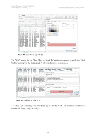
  • 137.
    CONDITIONAL FORMATTING AND CONDITIONALFORMULAS Conditional Formatting Formulas 137 Figure 256 - IF_AND_OR Functions (C) The colour settings have now been applied to the cell range cell A2 to cell E13. Figure 257 - IF_AND_OR Functions (D) If anyone needs support or assistance in creating formulas, using functions, and creating conditional formatting formulas, I have produced books and videos on creating formulas, using functions, and creating conditional formatting formulas. These products can be previewed and purchased by visiting the NILC Training website (www.nilc.co.uk).
  • 138.
    CONDITIONAL FORMATTING AND CONDITIONALFORMULAS Table of Figures 138 TABLE OF FIGURES Figure 1 – Conditional Formatting Example 9 Figure 2 - Greater Than (A) 10 Figure 3 - Greater Than (B) 11 Figure 4 - Greater Than (C) 11 Figure 5 - Greater Than (D) 11 Figure 6 - Greater Than (E) 12 Figure 7 - Greater Than (F) 12 Figure 8 - Less Than (A) 13 Figure 9 - Less Than (B) 13 Figure 10 - Less Than (C) 14 Figure 11 - Less Than (D) 14 Figure 12 - Less Than (E) 15 Figure 13 - Less Than (F) 15 Figure 14 - Between (A) 16 Figure 15 - Between (B) 17 Figure 16 - Between (C) 17 Figure 17 - Between (D) 18 Figure 18 - Between (E) 18 Figure 19 - Between (F) 19 Figure 20 - Equal To (A) 20 Figure 21 - Equal To (B) 20 Figure 22 - Equal To (C) 21 Figure 23 - Equal To (D) 21 Figure 24 - Equal To (E) 22 Figure 25 - Equal To (F) 22 Figure 26 - Text That Contains (A) 23 Figure 27 - Text That Contains (B) 23 Figure 28 - Text That Contains (C) 24 Figure 29 - Text That Contains (D) 24 Figure 30 - Text That Contains (E) 25 Figure 31 - Text That Contains (F) 25 Figure 32 - Date Occurring (A) 26 Figure 33 - Date Occurring (B) 27 Figure 34 - Date Occurring (C) 27 Figure 35 - Date Occurring (D) 28 Figure 36 - Date Occurring (E) 28 Figure 37 - Date Occurring (F) 29
  • 139.
    CONDITIONAL FORMATTING AND CONDITIONALFORMULAS Table of Figures 139 Figure 38 - Duplicate Values (A) 29 Figure 39 - Duplicate Values (B) 30 Figure 40 - Duplicate Values (C) 30 Figure 41 - Duplicate Values (D) 31 Figure 42 - Duplicate Values (E) 31 Figure 43 - Duplicate Values (F) 32 Figure 44 - Greater Than or Equal To (A) 32 Figure 45 - Greater Than or Equal To (B) 33 Figure 46 - Greater Than or Equal To (C) 33 Figure 47 - Greater Than or Equal To (D) 34 Figure 48 - Greater Than or Equal To (E) 34 Figure 49 - Greater Than or Equal To (F) 35 Figure 50 - Greater Than or Equal To (G) 35 Figure 51 - Less Than or Equal To (A) 36 Figure 52 - Less Than or Equal To (B) 36 Figure 53 - Less Than or Equal To (C) 37 Figure 54 - Less Than or Equal To (D) 37 Figure 55 - Less Than or Equal To (E) 38 Figure 56 - Less Than or Equal To (F) 38 Figure 57 - Less Than or Equal To (G) 39 Figure 58 - Blanks (A) 39 Figure 59 - Blanks (B) 40 Figure 60 - Blanks (C) 40 Figure 61 - Blanks (D) 41 Figure 62 - Blanks (E) 41 Figure 63 - Blanks (F) 42 Figure 64 - No Blanks (A) 42 Figure 65 - No Blanks (B) 43 Figure 66 - No Blanks (C) 43 Figure 67 - No Blanks (D) 44 Figure 68 - No Blanks (E) 44 Figure 69 - No Blanks (F) 45 Figure 70 - Errors (A) 45 Figure 71 - Errors (B) 46 Figure 72 - Errors (C) 46 Figure 73 - Errors (D) 46 Figure 74 - Errors (E) 47 Figure 75 - Errors (F) 47 Figure 76 - Errors (G) 48 Figure 77 - Top 10 Items (A) 49
  • 140.
    CONDITIONAL FORMATTING AND CONDITIONALFORMULAS Table of Figures 140 Figure 78 - Top 10 Items (B) 49 Figure 79 - Top 10 Items (C) 50 Figure 80 - Top 10 Item (D) 50 Figure 81 - Top 10 Items (E) 50 Figure 82 - Top 10 Items (F) 51 Figure 83 - Bottom 10 Items (A) 52 Figure 84 - Bottom 10 Items (B) 52 Figure 85 - Bottom 10 Items (C) 52 Figure 86 - Bottom 10 Items (D) 53 Figure 87 - Bottom 10 Items (E) 53 Figure 88 - Bottom 10 Items (F) 54 Figure 89 - Top 10% (A) 55 Figure 90 - Top 10% (B) 55 Figure 91 - Top 10% (C) 55 Figure 92 - Top 10% (D) 56 Figure 93 - Top 10% (E) 56 Figure 94 - Top 10% (F) 57 Figure 95 - Bottom 10% (A) 57 Figure 96 - Bottom 10% (B) 58 Figure 97 - Bottom 10% (C) 58 Figure 98 - Bottom 10% (D) 59 Figure 99 - Bottom 10% (E) 59 Figure 100 - Bottom 10% (F) 60 Figure 101 - Above Average (A) 61 Figure 102 - Above Average (B) 61 Figure 103 - Above Average (C) 61 Figure 104 - Above Average (D) 62 Figure 105 - Above Average (E) 62 Figure 106 - Above Average (F) 63 Figure 107 - Below Average (A) 64 Figure 108 - Below Average (B) 64 Figure 109 - Below Average (C) 64 Figure 110 - Below Average (D) 65 Figure 111 - Below Average (E) 65 Figure 112 - Below Average (F) 66 Figure 113 - Data Bars (A) 67 Figure 114 - Data Bars (B) 67 Figure 115 - Data Bars (C) 68 Figure 116 - Data Bars (D) 68 Figure 117 - Data Bars (E) 69
  • 141.
    CONDITIONAL FORMATTING AND CONDITIONALFORMULAS Table of Figures 141 Figure 118 - Data Bars (F) 69 Figure 119 - Data Bars (G) 70 Figure 120 - Data Bars (H) 70 Figure 121 - Data Bar No Values (A) 71 Figure 122 - Data Bar No Values (B) 71 Figure 123 - Data Bar No Values (C) 72 Figure 124 - Data Bar No Values (D) 72 Figure 125 - Data Bar No Values (E) 73 Figure 126 - Data Bar No Values (F) 73 Figure 127 - Data Bar No Values (G) 74 Figure 128 - Data Bar Negative Values (A) 74 Figure 129 - Data Bar Negative Values (B) 75 Figure 130 - Data Bar Negative Values (C) 75 Figure 131 - Data Bar Negative Values (D) 76 Figure 132 - Data Bar Negative Values (E) 76 Figure 133 - Data Bar Negative Values (F) 76 Figure 134 - Colour Scales (A) 77 Figure 135 - Colour Scales (B) 77 Figure 136 - Colour Scales (C) 78 Figure 137 - Colour Scales (D) 78 Figure 138 - Colour Scales (E) 79 Figure 139 - Colour Scales (F) 79 Figure 140 - Colour Scales Heat Map (A) 80 Figure 141 - Colour Scales Heat Map (B) 80 Figure 142 - Colour Scales Heat Map (C) 80 Figure 143 - Colour Scales Heat Map (D) 81 Figure 144 - Colour Scales Heat Map (E) 81 Figure 145 - Icon Sets (A) 82 Figure 146 - Icon Sets (B) 82 Figure 147 - Icon Sets (C) 83 Figure 148 - Icon Sets (D) 83 Figure 149 - Icon Sets (E) 84 Figure 150 - Icon Sets (F) 84 Figure 151 - Icon Sets (G) 85 Figure 152 - Icon Sets Positive/Negative Values (A) 85 Figure 153 - Icon Sets Positive/Negative Values (B) 86 Figure 154 - Icon Sets Positive/Negative Values (C) 86 Figure 155 - Icon Sets Positive/Negative Values (D) 87 Figure 156 - New Rule (A) 87 Figure 157 - New Rule (B) 88
  • 142.
    CONDITIONAL FORMATTING AND CONDITIONALFORMULAS Table of Figures 142 Figure 158 - New Rule (C) 88 Figure 159 - Manage Rules (A) 89 Figure 160 - Manage Rules (B) 89 Figure 161 - Manage Rules (C) 90 Figure 162 - Manage Rules (D) 90 Figure 163 - Manage Rules (E) 91 Figure 164 - Clearing Rules (A) 91 Figure 165 - Clearing Rules (B) 92 Figure 166 - Multiple Conditional Formatting (A) 92 Figure 167 - Multiple Conditional Formatting (B) 93 Figure 168 - Multiple Conditional Formatting (C) 93 Figure 169 - Multiple Conditional Formatting (D) 94 Figure 170 - Multiple Conditional Formatting (E) 94 Figure 171 - Multiple Conditional Formatting (F) 95 Figure 172 - Multiple Conditional Formatting (G) 95 Figure 173 - Multiple Conditional Formatting (H) 96 Figure 174 - Multiple Conditional Formatting (I) 96 Figure 175 - New Formatting Rule_ Using Formulas 97 Figure 176 - Absolute Cell Referencing (A) 98 Figure 177 - Absolute Cell Referencing (B) 99 Figure 178 - Absolute Cell Referencing (C) 99 Figure 179 - Relative Cell Referencing (A) 100 Figure 180 - Relative Cell Referencing (B) 100 Figure 181 - Relative Cell Referencing (C) 101 Figure 182 - Criteria Signs (A) 101 Figure 183 - Criteria Signs (B) 102 Figure 184 - Format Painter (A) 102 Figure 185 - Format Painter (B) 103 Figure 186 - Format Painter (C) 103 Figure 187 - Paste Special (A) 104 Figure 188 - Paste Special (B) 104 Figure 189 - Paste Special (C) 104 Figure 190 - Paste Special (D) 105 Figure 191 - Paste Special (E) 105 Figure 192 - Testing Conditional Formatting Formulas (A) 106 Figure 193 - True or False Testing (A) 106 Figure 194 - True or False Testing (B) 107 Figure 195 - Copying a Tested Formula (A) 107 Figure 196 - Copying a Tested Formula (B) 108 Figure 197 - Copying a Tested Formula (C) 108
  • 143.
    CONDITIONAL FORMATTING AND CONDITIONALFORMULAS Table of Figures 143 Figure 198 - Copying a Tested Formula (D) 109 Figure 199 - Copying a Tested Formula (E) 109 Figure 200 - Copying a Tested Formula (F) 110 Figure 201 - Copying a Tested Formula (G) 110 Figure 202 - Copying a Tested Formula (H) 111 Figure 203 - Controlling and Ordering Formatting (A) 111 Figure 204 - Controlling and Ordering Formatting (B) 112 Figure 205 - Controlling and Ordering Formatting (C) 112 Figure 206 - Controlling and Ordering Formatting (D) 113 Figure 207 - Controlling and Ordering Formatting (E) 113 Figure 208 - Controlling and Ordering Formatting (F) 114 Figure 209 - Controlling and Ordering Formatting (G) 114 Figure 210 - Controlling and Ordering Formatting (H) 115 Figure 211 - Controlling and Ordering Formatting (I) 115 Figure 212 - Managing Formula Formatting (A) 116 Figure 213 - Managing Formula Formatting (B) 116 Figure 214 - Managing Formula Formatting (C) 117 Figure 215 - Managing Formula Formatting (D) 117 Figure 216 - Managing Formula Formatting (E) 118 Figure 217 - Managing Formula Formatting (F) 118 Figure 218 - Managing Formula Formatting (G) 119 Figure 219 - Managing Formula Formatting (H) 119 Figure 220 - Managing Formula Formatting (I) 120 Figure 221 - Hiding Zero Values (A) 120 Figure 222 - Hiding Zero Values (B) 121 Figure 223 - Hiding Zero Values (C) 121 Figure 224 - Hiding Zero Values (D) 122 Figure 225 - Target Setting Formulas (A) 123 Figure 226 - Target Setting Formulas (B) 123 Figure 227 - Target Setting Formulas (C) 124 Figure 228 - Target Setting Formulas (D) 124 Figure 229 - Target Setting Formulas (E) 125 Figure 230 - Target Setting Formulas (F) 125 Figure 231 - Date Control Formulas (A) 126 Figure 232 - Date Control Formulas (B) 126 Figure 233 - Date Control Formulas (C) 126 Figure 234 - Date Control Formulas (D) 127 Figure 235 - Duplicate Rows Countifs (A) 127 Figure 236 - Duplicate Rows Countifs (B) 128 Figure 237 - Duplicate Rows Countifs (C) 128
  • 144.
    CONDITIONAL FORMATTING AND CONDITIONALFORMULAS Table of Figures 144 Figure 238 - Duplicate Rows Countifs (D) 128 Figure 239 - Highlighting Entire Rows (A) 129 Figure 240 - Highlighting Entire Rows (B) 129 Figure 241 - Highlighting Entire Rows (C) 130 Figure 242 - Highlighting Entire Rows (D) 130 Figure 243 - Highlighting Entire Rows (E) 131 Figure 244 - Highlighting Entire Rows (F) 131 Figure 245 - Highlighting Entire Rows (G) 132 Figure 246 - Highlighting Entire Rows (H) 132 Figure 247 - Highlighting Entire Rows (I) 133 Figure 248 - Highlighting Entire Rows (J) 133 Figure 249 - Highlighting Entire Rows (K) 134 Figure 250 - Highlighting Entire Rows (L) 134 Figure 251 - Standard Formula Formatting (A) 135 Figure 252 - Standard Formula Formatting (B) 135 Figure 253 - Standard Formula Formatting (C) 135 Figure 254 - IF_AND_OR Functions (A) 136 Figure 255 - IF_AND_OR Functions (B) 136 Figure 256 - IF_AND_OR Functions (C) 137 Figure 257 - IF_AND_OR Functions (D) 137