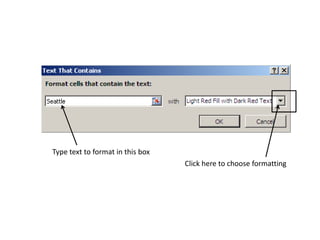
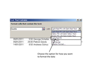
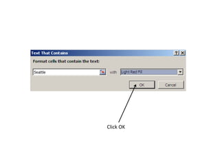
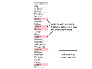
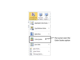
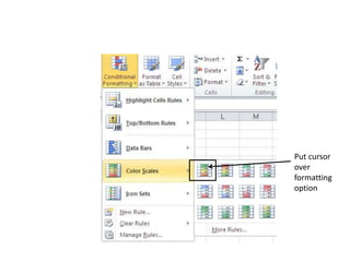
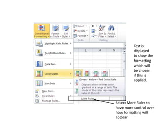
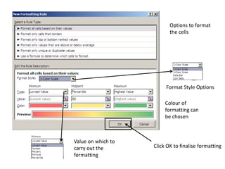
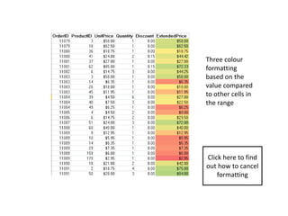
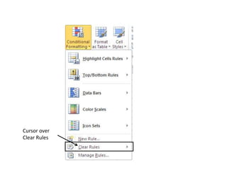
Conditional formatting in Excel allows cells to be formatted based on their data values. This makes spreadsheets easier to read. Formatting options include highlighting text that contains specific words, using color scales to shade cells differently based on values, and more granular controls over formatting styles and values. Conditional formatting rules can be cleared from a sheet by selecting "Clear Rules" under the Conditional Formatting menu.

1. Conditional formatting in Excel
Next Slide

2. Conditional Formatting
• Makes spreadsheets of complex data easier to
read by formatting cells based on the data
contained.
Next Slide

3. Highlight text in cells
Click here for Conditional
Formatting options
Home tab
Highlight column to
apply formatting to

4. Cursor over option
Highlight Cell Rules

5. As the column
contains
text, click Text
that Contains….

6. Type text to format in this box
Click here to choose formatting

7. Choose the option for how you want
to format the data

8. Click OK

9. All of the cells within the
highlighted range now have
the chosen formatting
Click here to go
to next example

10. Colour scales
Highlight
column you
wish to
format Click Conditional
Formatting

11. Put cursor over the
Color Scales option

12. Put cursor
over
formatting
option

13. Text is
displayed
to show the
formatting
which will
be chosen
if this is
applied.
Select More Rules to
have more control over
how formatting will
appear

14. Options to format
the cells
Format Style Options
Colour of
formatting can
be chosen
Value on which to
carry out the Click OK to finalise formatting
formatting

15. Three colour
formatting
based on the
value compared
to other cells in
the range
Click here to find
out how to cancel
formatting

16. Cancelling rules
Click Conditional
Formatting

17. Cursor over
Clear Rules

18. Select Clear
Rules from
Entire Sheet

19. Formatting on
the sheet
clears
Click
here to
end
show