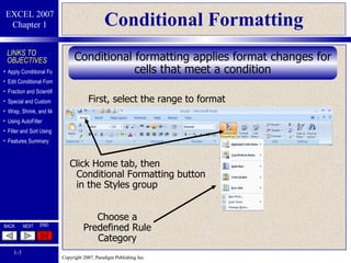
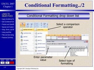
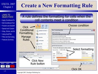
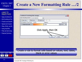
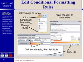
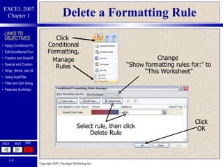
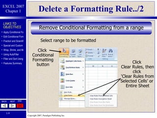
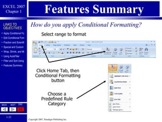
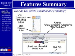
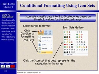
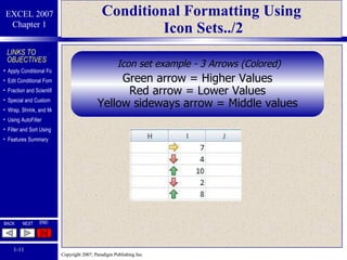
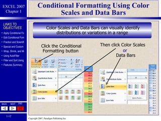
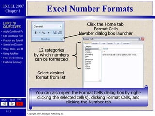
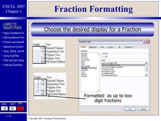
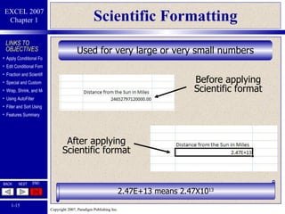
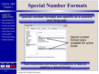
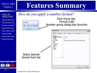
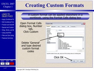
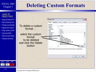
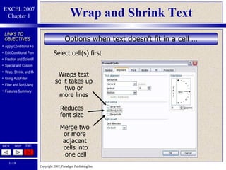
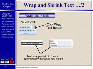
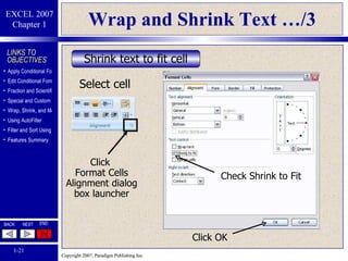
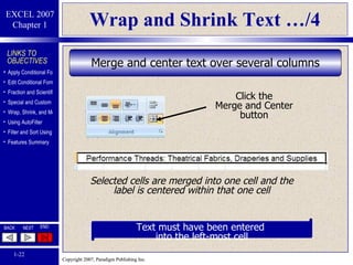
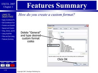
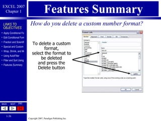
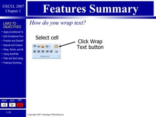
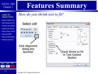
This document provides an overview of advanced formatting techniques in Microsoft Excel 2007, including: - Applying conditional formatting using predefined rules or custom rules. Creating, editing, and deleting conditional formatting rules. - Using conditional formatting options like icon sets, data bars, and color scales. Applying number, fraction, and scientific formatting. - Creating custom number formats. Applying wrap text and shrink to fit options. 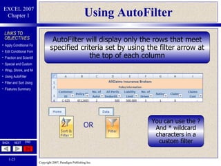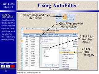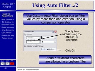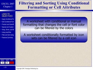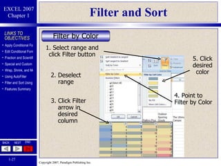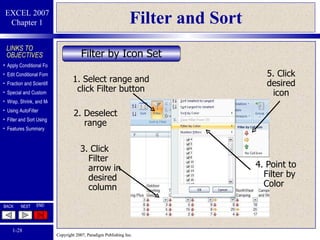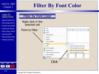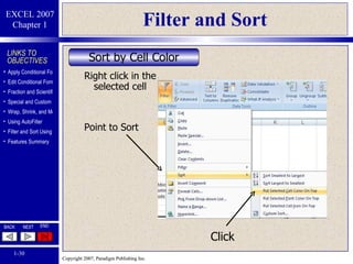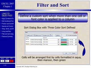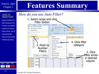- Using AutoFilter to filter a worksheet by values, colors, icons or other cell attributes. Filtering and sorting using conditional formatting. - Features for applying number formats, deleting custom formats, using AutoFilter, wrapping text, and shrinking text are summarized.

1. Microsoft Excel 2007 – Level 2 ADVANCED FORMATTING TECHNIQUES Chapter 1

2. Performance Objectives Apply conditional formatting by entering parameters for a rule Apply conditional formatting using a predefined rule Create and apply a new rule for conditional formatting Edit and delete a conditional formatting rule Apply conditional formatting using an icon set, data bars, and color scale Apply fraction and scientific formatting Apply a special format for a number Create a custom number format Apply wrap text and shrink to fit text control options Filter a worksheet using a custom Auto Filter Filter and sort a worksheet using conditional formatting Filter and sort a worksheet using cell attributes

3. Conditional Formatting Conditional formatting applies format changes for cells that meet a condition Click Home tab, then Conditional Formatting button in the Styles group Choose a Predefined Rule Category First, select the range to format

4. Conditional Formatting../2 Conditional Formatting drop down list Select a comparison operator Enter parameter value Select type of formatting

5. Create a New Formatting Rule A rule defines the formatting for cells when the cell contents meet a condition Click Conditional Formatting, Manage Rules Click New Rule button Choose condition Select formatting Click OK

6. Create a New Formatting Rule …/2 Click Apply, then OK Create a rule to format cells based on values, text, dates, blank or error values

7. Edit Conditional Formatting Rules Select range to format Click Conditional Formatting, Manage Rules Click desired rule, then Edit Rule Make changes to parameters Click OK

8. Delete a Formatting Rule Click Conditional Formatting, Manage Rules Change “Show formatting rules for:” to “This Worksheet” Select rule, then click Delete Rule Click OK

9. Delete a Formatting Rule../2 Remove Conditional Formatting from a range Select range to be formatted Click Conditional Formatting button Click Clear Rules, then click ‘Clear Rules from Selected Cells’ or Entire Sheet

10. Conditional Formatting Using Icon Sets Icon sets classify data into 3 to 5 categories based on threshold values for the selected range Select range to format Click Conditional Formatting, Icon Sets Click the Icon set that best represents the categories in the range Icon Sets Gallery

11. Conditional Formatting Using Icon Sets../2 Icon set example - 3 Arrows (Colored) Green arrow = Higher Values Red arrow = Lower Values Yellow sideways arrow = Middle values

12. Conditional Formatting Using Color Scales and Data Bars Color Scales and Data Bars can visually identify distributions or variations in a range Click the Conditional Formatting button Then click Color Scales or Data Bars

13. Excel Number Formats 12 categories by which numbers can be formatted Click the Home tab, Format Cells Number dialog box launcher You can also open the Format Cells dialog box by right-clicking the selected cell(s), clicking Format Cells, and clicking the Number tab Select desired format from list

14. Fraction Formatting Choose the desired display for a Fraction Formatted as up to two digit fractions

15. Scientific Formatting Used for very large or very small numbers Before applying Scientific format After applying Scientific format 2.47E+13 means 2.47X10 13

16. Special Number Formats Special number formats are specific to a country and language Special number format types available for active locale Save keystrokes and ensure consistency of data by applying a special format

17. Creating Custom Formats Delete ‘General’ and type desired custom format codes Click OK A custom format can be applied elsewhere in a workbook, using the Format Cells dialog box Open Format Cells dialog box, Number tab, Click Custom

18. Deleting Custom Formats To delete a custom format … select the custom format to be deleted and click the Delete button

19. Wrap and Shrink Text Options when text doesn’t fit in a cell … Wraps text so it takes up two or more lines Reduces font size Merge two or more adjacent cells into one cell Select cell(s) first

20. Wrap and Shrink Text …/2 Wrap text in cells Text wrapped within the cell automatically increases row height Click Wrap Text button Select cell

21. Wrap and Shrink Text …/3 Shrink text to fit cell Click Format Cells Alignment dialog box launcher Select cell Check Shrink to Fit Click OK

22. Wrap and Shrink Text …/4 Click the Merge and Center button Selected cells are merged into one cell and the label is centered within that one cell Merge and center text over several columns Text must have been entered into the left-most cell

23. Using AutoFilter AutoFilter will display only the rows that meet specified criteria set by using the filter arrow at the top of each column You can use the ? And * wildcard characters in a custom filter OR

24. Using AutoFilter 1. Select range and click Filter button 2. Click Filter arrow in desired column 4. Click filter category 3. Point to Number Filters

25. Using Auto Filter../2 Use Custom Auto Filter dialog box to filter values by more than one criterion using a comparison operator Specify two criteria using the AND or OR operators ? and * wildcard characters are allowed in a custom filter Click OK

26. Filtering and Sorting Using Conditional Formatting or Cell Attributes A worksheet with conditional or manual formatting that changes the cell or font color can be filtered by the colors A worksheet conditionally formatted by icon sets can be filtered by a cell icon

27. Filter and Sort 1. Select range and click Filter button 3. Click Filter arrow in desired column 2. Deselect range 4. Point to Filter by Color 5. Click desired color Filter by Color

28. Filter and Sort 1. Select range and click Filter button 3. Click Filter arrow in desired column 2. Deselect range 4. Point to Filter by Color 5. Click desired icon Filter by Icon Set

29. Filter By Font Color Right click in the selected cell Point to Filter Filter by Font Color Click

30. Filter and Sort Right click in the selected cell Point to Sort Sort by Cell Color Click

31. Filter and Sort Define a custom sort when more than one cell or font color is applied to a column Cells will be arranged first by cells formatted in aqua, then maroon, then green Sort Dialog Box with Three Color Sort Defined

32. Features Summary How do you apply Conditional Formatting? Click Home Tab, then Conditional Formatting button Choose a Predefined Rule Category Select range to format

33. Features Summary How do you delete Conditional Formatting? Click Conditional Formatting button Click Manage Rules Change “Show formatting Rules for” to “This Worksheet” Click OK Select rule, then click Delete Rule

34. Features Summary How do you create a custom format? Delete “General” and type desired custom format codes Click OK

35. Features Summary How do you apply a number format? Select desired format from list Click Home tab, Format Cells Number group dialog box launcher

36. Features Summary How do you delete a custom number format? To delete a custom format, select the format to be deleted and press the Delete button

37. Features Summary How do you use Auto Filter? 1. Select range and click Filter button 2. Click Filter arrow in desired column 4. Click filter category 3. Point to Number Filters

38. Features Summary How do you wrap text? Click Wrap Text button Select cell

39. Features Summary How do you shrink text to fit? Select cell Check Shrink to Fit in Text Control Section Click Alignment dialog box launcher

40. Coming Next ADVANCED FUNCTIONS AND FORMULAS Chapter 2