Microsoft Excel Tutorial

YOU WILL LEARN ABOUT:
CHART
CONDITIONAL FORMATTING
PIVOT TABLES
FUNCTIONS
RELATIVE & ABSOLUTE CELL
REFERENCES

YOU WILL LEARN ABOUT:
COMPLEX FORMULAS
IF FUNCTION
VLOOKUP
CONCATENATE
COUNTA & COUNTIF

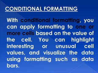
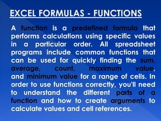
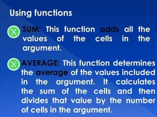
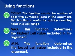
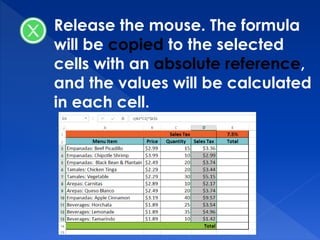
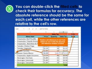
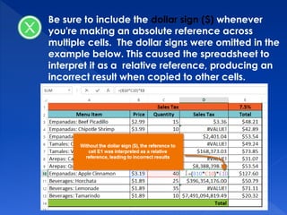
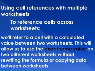
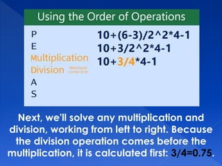
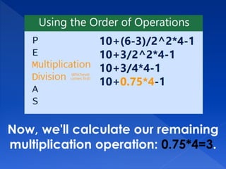
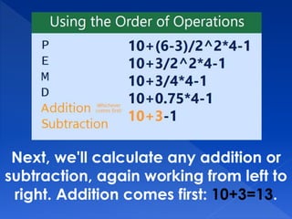
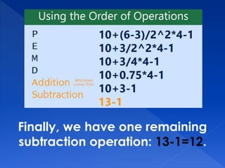
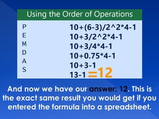
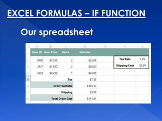
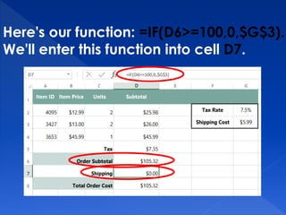
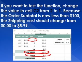
Excel is a computer program used to
create electronic spreadsheets.
Excel user can organize data, create
chart and perform calculation.
Excel is a convenient program because it
allow user to create large spreadsheets,
reference information and it allows for
better storage of information.

CHART
A chart is a tool you can use in
Excel to communicate your data
graphically. Charts allow your
audience to more easily see the
meaning behind the numbers in
the spreadsheet, and to make
showing comparisons and trends
much easier.

To create a chart:
Select the worksheet you want
to work with.
Select the cells you want to
chart, including the column
titles and row labels.

Hover over each Chart
option in the Charts group to
learn more about it.
Select one of the Chart options.
In this example, we'll use the
Columns command.
Click the Insert tab.

Select a type of chart from the
list that appears. For this
example, we'll use a 2-D
Clustered Column. The chart
appears in the worksheet.

Identifying the parts of a chart
Charts are a visual representation of
data in a worksheet. Charts make it
easy to see comparisons, patterns,
and trends in the data.

Chart tools
Once you insert a chart, a new
set of Chart Tools, arranged into
three tabs, will appear above
the Ribbon. These are only
visible when the chart is
selected.

To change the chart type:
Select the Design tab.
Click the Change Chart
Type command. A dialog
box appears.

Select another chart type.
Click OK.
The chart in the example compares each
salesperson's monthly sales to his or her other
months' sales; however, you can change what is
being compared. Just click the Switch
Row/Column Data command, which will rotate
the data displayed on the x and y axes. To
return to the original view, click the Switch
Row/Column command again.

To change chart layout:
Locate the Chart Layouts
group
Click the More arrow to
view all of your layout
options.

Left-click a layout to select it.
If your new layout includes chart
titles, axes, or legend labels, just
insert your cursor into the text and
begin typing to add your own text.

To change chart style:
Locate the Chart
Style group.
Click the More arrow to
view all of your style
options.

Left-click a style to select it.

To move the chart to a different
worksheet:
Click the Move
Chart command. A dialog
box appears. The current
location of the chart is
selected.

Select the desired location
for the chart (i.e., choose
an existing worksheet, or
select New Sheet and
name it).

CONDITIONAL FORMATTING
With conditional formatting, you
can apply formatting to one or
more cells based on the value of
the cell. You can highlight
interesting or unusual cell
values, and visualize the data
using formatting such as data
bars.

The conditional formatting options
Highlight cell rules

If you might want to see
order amounts greater than
300. Highlight Order Amount
from top to bottom then
select Greater Than..
Select OK

If you might want to see
Top/Bottom 10 order
amounts. Highlight Order
Amount from top to bottom
then select Top 10 items..
Select OK

This is an interesting option that formats
the selected cells with colored bars.
The length of the data bar represents
the value in the cell. The longer the
bar, the higher the value.

Color Scales
Select
by
clicking

This option applies a two- or three-
color gradient to the cells. Different
shades and colors represent specific
values.

To apply conditional formatting:
Select the cells you would
like to format.
Select the Home tab.
Locate the Styles group.

Click the Conditional
Formatting command. A
menu will appear with your
formatting options

Select one of the options to
apply it to the selected cells.
A cascading menu will
appear.

An additional
dialog box
may appear,
depending on
the option
you choose.
If so, make the
necessary
choices, then
click OK.

To remove conditional formatting
rules:
Formatting command.
Select Clear Rules. A
cascading menu appears.

Choose to
clear rules
from
the entire
worksheet or
the selected
cells.

To manage conditional formatting
rules:
Formatting command.
Select Manage Rules from
the menu. The Conditional
Formatting Rules Manager
dialog box will appear.

From here you can edit a
rule, delete a rule, or
change the order of rules.

PIVOT TABLES
PivotTable reports, or PivotTables as they are
often called, can help you answer questions
about your spreadsheet by analyzing the
numerical information in various ways. If you
work with spreadsheets with a lot of data, a
PivotTable can be an extremely useful tool.
PivotTable reports give you power because
you can quickly find the answer to many
different questions and can manipulate your
data in many different ways.

To Create PivotTable
Select
the
Insert
Tab

Select a table or
range is already
selected, and
the Table/Range
field shows the
range of the
selected data.
New Worksheet is
also selected by
default as the
place where the
report will be
placed.

When you create a
PivotTable,
each column
label in your data
becomes a
field that can be
used in the report.
The Field
List appears on the
right side of the
report, while the
layout
area appears on
the left.

In this
Company
Sales Report
you might
want to
know which
salesperson
sold the
highest dollar
amount.

Select the
checkbox
Smith, Bob is the
top salesman

If you change any of the data
in your source worksheet, the
PivotTable will not update
automatically. To manually
update it, select the PivotTable
and then go to Options
Refresh.

To add a report filter
Select a field in the Field List. In
this example, choose Region.
By default, it will appear in the
Row Labels group.

Click and
drag Region into
the Report
Filter section.
Release the mouse
button. The region
appears at the top
of the report as a
filter.

The arrow by the Region fields shows (All).
To show just the data for a specific region,
click the drop-down arrow, and select
the region. To see multiple regions, click
the Multiple Regions box, select the
regions to display, then click OK.

If you might want to see who is the
salesman in East Region just select East.
Click OK

To move or pivot data
Release the mouse button to drop the
field in the new area. In this example, we
move Region from Report Filter to Column
Label. The PivotTable report will change.

Right-click one of the rows. A
menu will appear.
Select Move, then select a
move option.

To create a PivotChart
Select the PivotChart command
from the Options tab. The Insert
Chart dialog box appears.

Select the chart you’d like to
insert.
Click OK. The chart will now
appear on the same sheet as
the PivotTable.

EXCEL FORMULAS - FUNCTIONS
A function is a predefined formula that
performs calculations using specific values
in a particular order. All spreadsheet
programs include common functions that
can be used for quickly finding the sum,
average, count, maximum value,
and minimum value for a range of cells. In
order to use functions correctly, you'll need
to understand the different parts of a
function and how to create arguments to
calculate values and cell references.

The parts of a function
In order to work correctly, a
function must be written a
specific way, which is called
the syntax.

The basic
syntax for a
function
one or
more arguments
contain the information
you want to calculate
The function in the example below would
add the values of the cell range A1:A20

Working with arguments
Arguments can refer to
both individual
cells and cell
ranges and must be
enclosed
within parentheses.
You can include one
argument or multiple
arguments, depending
on the syntax required
for the function.

For example, the
function =AVERAGE
(B1:B9) would
calculate
the average of the
values in the cell
range B1:B9.
This function
contains only one
argument.

Multiple arguments must be
separated by a comma. For
example, the function =SUM(A1:A3,
C1:C2, E2) will add the values of all
cells in the three arguments.

Using functions
SUM: This function adds all the
values of the cells in the
argument.
AVERAGE: This function determines
the average of the values included
in the argument. It calculates
the sum of the cells and then
divides that value by the number
of cells in the argument.

Using functions
COUNT: This function counts the number of
cells with numerical data in the argument.
This function is useful for quickly counting
items in a cell range.
MAX: This function determines
the highest cell value included in the
argument.
MIN: This function determines
the lowest cell value included in the
argument.

To use a function:
Select the cell that will contain
the function. In our example,
we'll select cell C11.

Type the equals sign (=) and
enter the desired function name.
In our example, we'll
type =AVERAGE.

Enter the cell range for
the argument inside parentheses. In our
example, we'll type (C3:C10). This formula
will add the values of cells C3:C10 and
then divide that value by the total number
of cells in the range to determine the
average.

Press Enter on your keyboard. The function
will be calculated, and the result will
appear in the cell. In our example, the
average price per unit of items ordered
was $15.93.

EXCEL FORMULAS - RELATIVE AND
ABSOLUTE CELL REFERENCES
Relative references change when
a formula is copied to another cell.
Absolute references, on the other
hand, remain constant no matter
where they are copied.

To create and copy a formula
using relative references:
Relative references

the formula. In our example,
we'll select cell D2.

Enter the formula to calculate
the desired value. In our
example, we'll type =B2*C2.

Press Enter on your keyboard.
The formula will be calculated,
and the result will be displayed
in the cell.

Locate the fill handle in the
lower-right corner of the
desired cell. In our example,
we'll locate the fill handle for
cell D2.

Click, hold, and drag the fill
handle over the cells you wish
to fill. In our example, we'll
select cells D3:D12.

Release the mouse. The formula
will be copied to the selected
cells with relative references and
the values will be calculated in
each cell.

You can double-click the filled cells to
check their formulas for accuracy. The
relative cell references should be
different for each cell, depending on
its row.

Absolute references
An absolute reference is
designated in a formula by the
addition of a dollar sign ($). It can
precede the column reference,
the row reference, or both.

You will usually use
the $A$2 format when creating
formulas that contain absolute
references.
When writing a formula in
Microsoft Excel, you can press
the F4 key on your keyboard
to switch between relative and
absolute cell references.

To create and copy a formula
using absolute references:

In our example, we'll use the 7.5%
sales tax rate in cell E1 to
calculate the sales tax for all items
in column D. We'll need to use the
absolute cell reference $E$1 in our
formula. Because each formula is
using the same tax rate, we want
that reference to remain constant
when the formula is copied and
filled to other cells in column D.

the formula. In our example,
we'll select cell D3.

Enter the formula to calculate
the desired value. In our
example, we'll type
=(B3*C3)*$E$1.

The formula will calculate,
and the result will display in
the cell.

Locate the fill handle in the lower-
right corner of the desired cell. In
our example, we'll locate the fill
handle for cell D3.

Click, hold, and drag the fill
handle over the cells you wish
to fill, cells D4:D13 in our
example.

Release the mouse. The formula
will be copied to the selected
cells with an absolute reference,
and the values will be calculated
in each cell.

You can double-click the filled cells to
check their formulas for accuracy. The
absolute reference should be the same for
each cell, while the other references are
relative to the cell's row.

Be sure to include the dollar sign ($) whenever
you're making an absolute reference across
multiple cells. The dollar signs were omitted in the
example below. This caused the spreadsheet to
interpret it as a relative reference, producing an
incorrect result when copied to other cells.

Using cell references with multiple
worksheets
To reference cells across
worksheets:
we'll refer to a cell with a calculated
value between two worksheets. This will
allow us to use the exact same value on
two different worksheets without
rewriting the formula or copying data
between worksheets.

Locate the cell you wish to reference,
and note its worksheet. In our
example, we want to reference
cell E15 on the Menu Order
worksheet.

Navigate to the desired worksheet.
In our example, we'll select
the Catering Invoice worksheet.

The selected worksheet will appear.
Locate and select the cell where you
want the value to appear. In our
example, we'll select cell B3.

Type the equals sign (=), click Menu
Order Sheet

Select the value you want to appear
on other sheet, select E15

The value of the referenced cell will
appear.

If the value of cell E15 changes
on the Menu Order worksheet, it
will be updated automatically on
the Catering Invoice worksheet.
If you rename your worksheet at
a later point, the cell reference
will be updated automatically to
reflect the new worksheet name.

EXCEL FORMULAS - COMPLEX
FORMULAS
A complex formula has more than
one mathematical operator, such
as 5+2*8. When there is more than
one operation in a formula, the order
of operations tells your spreadsheet
which operation to calculate first. In
order to use complex formulas, you
will need to understand the order of
operations.

The order of operations
All spreadsheet programs
calculate formulas based on the
following order of operations:
1. Operations enclosed
in parentheses
2. Exponential calculations
(3^2, for example)

3. Multiplication and division,
whichever comes first
4. Addition and subtraction,
whichever comes first
A mnemonic that can help you
remember the order is PEMDAS,
or Please Excuse My Dear Aunt Sally.

While this formula may look really
complicated, we can use the order of
operations step by step to find the right
answer.

First, we'll start by calculating anything
inside the parentheses. In this case,
there's only one thing we need to
calculate: 6-3=3.

As you can see, the formula already
looks a bit simpler. Next, we'll look to
see if there are any exponents. There's
one: 2^2=4.

Next, we'll solve any multiplication and
division, working from left to right. Because
the division operation comes before the
multiplication, it is calculated first: 3/4=0.75.

Now, we'll calculate our remaining
multiplication operation: 0.75*4=3.

Next, we'll calculate any addition or
subtraction, again working from left to
right. Addition comes first: 10+3=13.

Finally, we have one remaining
subtraction operation: 13-1=12.

And now we have our answer: 12. This is
the exact same result you would get if you
entered the formula into a spreadsheet.

EXCEL FORMULAS – IF FUNCTION
Our spreadsheet

How can we solve this problem?
If the subtotal for an order is at
least $100, the shipping should
be free. If not, it should cost
$5.99. We could use
the IF function to solve this
problem.

Writing the function
The first argument sets up the
condition the IF function will test:
In this example, if the value in cell
D6 is greater than or equal to 100.
So our first argument will
be D6>=100.

The second argument tells the
function what to write if the
condition is true. In this example,
if the value is greater than or
equal to 100, we want it to write
"0" in the cell. So our second
argument will be 0.

The third argument tells the
function what to write if the
condition is false: In this example,
if the value is less than 100, we
want it to use the value from cell
G3 (5.99). So our third argument
will be $G$3 (we'll use an
absolute reference here just in
case we move this formula in the
future).

Here's our function: =IF(D6>=100,0,$G$3).
We'll enter this function into cell D7.

If you want to test the function, change
the value in cell C2 from 2 to 1. Because
the Order Subtotal is now less than $100,
the Shipping cost should change from
$0.00 to $5.99.

EXCEL FORMULAS – VLOOKUP
Our spreadsheet

What are we trying to do with this
spreadsheet?
Use the Product ID number to find
the product name and price from
the Products worksheet. Luckily,
the VLOOKUP function can do this
automatically.

How it works
it will search for the Product ID number
on the Products worksheet. It first
searches vertically down the first
column (VLOOKUP is short for "vertical
lookup"). When it finds the desired
product ID, it moves to the right to find
the product name and product price.

The arguments will tell VLOOKUP what to
search for and where to look. We'll need
to use four arguments:
The first argument tells
VLOOKUP what to search for.
In our example, we're
searching for the product ID
number, which is in cell A2, so
our first argument is A2.

The second argument is a cell
range that tells VLOOKUP where to
look for the value from our first
argument. In our example, we want
it to search for this value in cell
range A2:C13 on the Products
worksheet, so our second argument
is Products!$A$2:$C$13. Note that
we're using absolute references so
this range won't change when we
copy the formula to other cells.

The third argument is the column
index number, which is simpler than
it sounds: The first column in the cell
range from the previous argument
is 1, the second column is 2, and so
on. In our example, we're looking
for the Product Name. The names
are stored in the second column of
the cell range from the previous
argument, so our our third
argument is 2.

The fourth argument tells
VLOOKUP if it should look
for approximate or exact match
es. If it is TRUE, it will look for
approximate matches. If it
is FALSE, it will look for exact
matches. In this example, we're
only looking for exact matches,
so our fourth argument is FALSE.

It's important to know that
VLOOKUP will always search
the leftmost column in the cell
range. Since our cell range
is A2:C13, it will
search column A.

Now that we have our
arguments, we'll write our
function in cell B2. We'll start
by typing an equals sign (=),
followed by the function
name and an open
parenthesis:

=VLOOKUP(
Next, we'll add each of the
four arguments, separate
them with commas, then
close the parentheses:
=VLOOKUP(A2,
Products!$A$2:$C$13, 2,
FALSE)

Note: Be sure to type the product
ID exactly as it appears above, with
no spaces. Otherwise, the VLOOKUP
function will not work correctly.

Adding the product price
Next, we also want the Product ID to
pull in the product price, so we'll use
the VLOOKUP function again. Since
we're using the same data, this
function will be very similar to the one
we just added. In fact, all we have to
do is change the third argument to 3.
This will tell VLOOKUP to pull in the
data from the third column, where the
product price is stored:

=VLOOKUP(A2,
Products!$A$2:$C$13, 3,
FALSE)

We've got our formulas
working, so we can just select
cells B2 and C2 and then drag
the fill handle down to copy
the formulas to the other rows
in the invoice. Now, each row
is using VLOOKUP to find the
Product Name and Product
Price.

EXCEL FORMULAS – CONCATENATE
Our spreadsheet

How can we solve this
problem quickly?
We want the information from the Last
Name and First Name column to appear
together in the same cell, but it would
take a long time to type everything by
hand. Rather than combining this data
manually, we can use the
CONCATENATE function to do it
automatically.

How it works
The word concatenate is just another
way of saying "to combine" or "to join
together". The CONCATENATE function
allows you to combine text from
different cells into one cell. In our
example, we can use it to combine
the text in column A and column B to
create a combined name in a new
column.

Before we start writing the function,
we'll need to insert a new column in
our spreadsheet for this data. In our
example, we'll insert it to the right of
column B.

=CONCATENATE(B2, A2)

To add a space, we can
simply add another
argument: " " (two double
quotes around a space).
Make sure the three
arguments are separated by
commas:
=CONCATENATE(B2," ",A2)

Perfect! Now we can use the fill
handle to copy the formula to the
remaining cells in this column.

EXCEL TIPS – COUNTA & COUNTIF
Our spreadsheet

Counting responses
=COUNTA(C2:C100)

Counting invitees
=COUNTA(A2:A100)

Counting invitees responded
with YES
=COUNTIF(C2:C86,E6)

Counting invitees responded
with NO
=COUNTIF(C2:C86,E7)

Microsoft Excel Tutorial

Recommended

Recommended

More Related Content

What's hot

What's hot (20)

Similar to Microsoft Excel Tutorial

Similar to Microsoft Excel Tutorial (20)

More from Kristine Tiongco-Rimpa

More from Kristine Tiongco-Rimpa (10)

Recently uploaded

Recently uploaded (20)

Microsoft Excel Tutorial