Download as PDF, PPTX
![The problem
y (x) = f (x, y(x)),
y(x0) = y0,
(1)
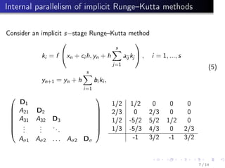
where x ∈ [x0; X], y ∈ Rm.
Gear classification:
1 parallelism across the system or, that is the same, parallelism across
the space;
2 parallelism across the method or, that is the same, parallelism across
the time.
2 / 14](https://image.slidesharecdn.com/parode-161008152319/85/Parallel-Numerical-Methods-for-Ordinary-Differential-Equations-a-Survey-2-320.jpg)
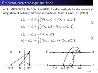

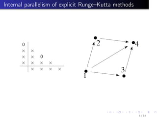
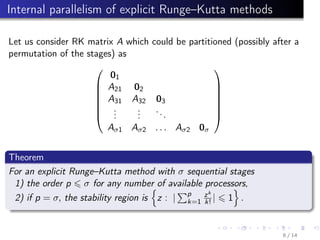

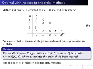


This document summarizes parallel numerical methods for solving ordinary differential equations (ODEs). It discusses two types of parallelism: across the system (space) and across the method (time). Predictor-corrector and Runge-Kutta methods are described that can exploit parallelism across time by parallelizing stages. Optimal Runge-Kutta methods use the minimum number of stages for a given order. Block methods solve ODE systems in parallel. Extrapolation and multiple shooting methods are also mentioned for parallelizing ODE solutions.