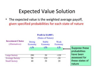
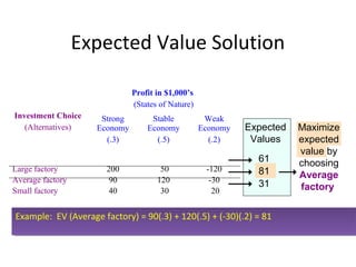
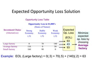
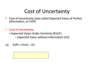
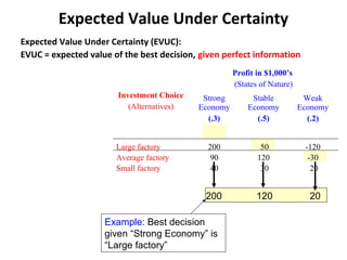
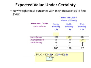
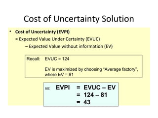
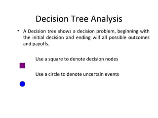
Operations Research Techniques
Introduction
• Operations Research is an Art and Science
• It had its early roots in World War II and is flourishing in
business and industry with the aid of computer
• Primary applications areas of Operations Research include
forecasting, production scheduling, inventory control,
capital budgeting, and transportation.
Operations Research
• “Operational Research is the scientific study of
operations for the purpose of making better
decisions.”
Terminology
• The British/Europeans refer to “Operational Research",
the Americans to “Operations Research" - but both are
often shortened to just "OR".
• Another term used for this field is “Management Science"
("MS"). In U.S. OR and MS are combined together to form
"OR/MS" or "ORMS".
• Yet other terms sometimes used are “Industrial
Engineering" ("IE") and “Decision Science" ("DS").
History of OR
 Operational Research has been existed as a science since
1930‘s.
 But as a formal discipline Operational Research originated
by the efforts of military planner during World War II .
In the decade after World War-II the techniques began to
be applied more widely in problems of business, industries
and societies.
Objectives
 Decision making and improve its quality.
• Identify optimum solution.
• Integrating the systems.
• Improve the objectivity of analysis.
• Minimize the cost and maximize the profit.
• Improve the productivity.
• Success in competition and market leadership.
Applications of OR
1. Finance and Accounting:
a. Dividend policies, investment and portfolio
management, auditing, balance sheet
b. Claim and Complaint procedure and public accounting
c. Break-even analysis, capital budgeting, cost allocation
and control, and financial planning
2. Marketing
• Selection of product mix
• Marketing and export planning
• Sales force allocations
• Assignment allocations
• Media planning
• Advertising
3. Purchasing & Procurement
• Optimal buying
• Transportation planning
• Replacement policies
• Bidding Policies
• Vendor analysis
4.Production management
• Facility location
• Logistics arrangement
• Layout design
• Engineering design
• Aggregate production planning
• Transportation
• Planning and scheduling
5. Personnel Management
• Manpower planning
• Wage/ salary administration
• Negotiation in bargaining situation
• Skills and Wages Balancing
• Schedule of training programmes
• Skill development and retention
6. General Management
• Decision Support system
• Forecasting
• Making quality control more effective
• Project Management and strategic planning
methods
Most projects of Operational Research apply
one of three broad groups of methods :-
1.Simulation methods.
2.Optimization methods.
3.Data-analysis methods.
1.Simulation methods
It gives ability to conduct sensitive study to -
(a). search for improvements and
(b). test the improvement ideas that are being made.
2.Optimization methods.
 Here goal is to enable the decision makers to identify and locate the
very best choice, where innumerable feasible choices are available
and comparing them is difficult.
3.Data-analysis methods
 The goal is to aid the decision-maker in detecting actual patterns and
inter-connections in the data set and
 Use of this analysis for making solutions.
 This method is very useful in Public Health.
Deterministic vs. Stochastic Models
Deterministic models (Non-Probabilistic)
assume all data are known with certainty
Stochastic models (Probabilistic Models)
explicitly represent uncertain data via
random variables or stochastic processes.
Deterministic models involve optimization
Stochastic models
characterize / estimate system performance.
Operations Research Models
Deterministic Models Stochastic Models
• Linear Programming • Discrete-Time Markov
Chains
• Network Optimization • Continuous-Time Markov
Chains
• Integer Programming • Queuing Theory (waiting
lines)
• Nonlinear Programming • Decision Analysis
Process
1. Identification of program problem.
 Most critical step in the process.
 Unless problem is clearly defined it is impossible
to develop good solutions.
2: Identification of possible reasons and solutions .
 Once the problem has been identified , it is the
job of the program implementer and researcher
to determine the reasons for the problem and
generate possible solutions.
3.Testing of potential solution
 A good solution must be measurable, easy to implement and sustainable.
 To determine effectiveness of proposed solution two designs are used-
(a) quasi-experimental design.
- comparison of situations before and after the solution.
(b) true experiment.
- comparison of outcome between experimental and control groups.
4.Result utilization
 It is necessary to decide how its results are meant to be used.
 This determine to some extent that what information should be collected.
5.Results dissemination
Results dissemination are done in the form of seminars or by meeting with decision makers.
Examples of OR Applications
• Rescheduling aircraft in response to groundings and
delays
• Planning production for printed circuit board assembly
• Scheduling equipment operators in mail processing &
distribution centers
• Developing routes for propane delivery
• Adjusting nurse schedules in light of daily fluctuations in
demand
Introduction to Decision Analysis
Decision Making Overview
Decision Making
Certainty Nonprobabilistic
Uncertainty Probabilistic
Decision Environment Decision Criteria
The Decision Environment
Certainty
Uncertainty
Decision Environment
Certainty: The results of decision alternatives
are known
Decision Making Under Certainty When it is
known for certain which is of the possible
future conditions will happen, just choose the
alternative that has the best payoff under the
state of nature
Example:
Must print 10,000 color brochures
Offset press A: 2,000 fixed cost
+ 0.24 per page
Offset press B: 3,000 fixed cost
+ 0.12 per page
*
The Decision Environment
Uncertainty
Certainty
Decision Environment
Uncertainty: The outcome that will occur
after a choice is unknown
Example:
You must decide to buy an item now or wait.
If you buy now the price is 2,000. If you wait
the price may drop to 1,500 or rise to 2,200.
There also may be a new model available
later with better features.
*
Decision Criteria
Nonprobabilistic
Probabilistic
Decision CriteriaNonprobabilistic Decision Criteria: Decision
rules that can be applied if the probabilities of
uncertain events are not known.
*
 maximax criterion
 maximin criterion
 minimax regret criterion
Decision Criteria
Nonprobabilistic
Probabilistic
Decision Criteria
*
Probabilistic Decision Criteria: Consider the
probabilities of uncertain events and select
an alternative to maximize the expected
payoff of minimize the expected loss
 maximize expected value
 minimize expected opportunity loss
PAYOFF
• The payoffs of a decision analysis
problem are the benefits or rewards that
result from selecting a particular decision
alternative
A Payoff Table
A payoff table shows alternatives, states of nature,
and payoffs
Investment
Choice
(Alternatives)
Profit in $1,000’s
(States of Nature)
Strong
Economy
Stable
Economy
Weak
Economy
Large factory
Average factory
Small factory
200
90
40
50
120
30
-120
-30
20
Maximax Solution
Investment
Choice
(Alternatives)
Profit in $1,000’s
(States of Nature)
Strong
Economy
Stable
Economy
Weak
Economy
Large factory
Average factory
Small factory
200
90
40
50
120
30
-120
-30
20
1.
Maximum
Profit
200
120
40
The maximax criterion (an optimistic approach):
1. For each option, find the maximum payoff
Maximax Solution
Investment
Choice
(Alternatives)
Profit in $1,000’s
(States of Nature)
Strong
Economy
Stable
Economy
Weak
Economy
Large factory
Average factory
Small factory
200
90
40
50
120
30
-120
-30
20
1.
Maximum
Profit
200
120
40
The maximax criterion (an optimistic approach):
1.For each option, find the maximum payoff
2.Choose the option with the greatest maximum payoff
2.
Greatest
maximum
is to
choose
Large
factory
(continued)
Maximin Solution
Investment
Choice
(Alternatives)
Profit in $1,000’s
(States of Nature)
Strong
Economy
Stable
Economy
Weak
Economy
Large factory
Average factory
Small factory
200
90
40
50
120
30
-120
-30
20
1.
Minimum
Profit
-120
-30
20
The maximin criterion (a pessimistic approach):
1. For each option, find the minimum payoff
2. Choose the option with the greatest minimum payoff
2.
Greatest
minimum
is to
choose
Small
factory
Opportunity Loss
Investment Choice
(Alternatives)
Profit in $1,000’s
(States of Nature)
Strong
Economy
Stable
Economy
Weak
Economy
Large factory
Average factory
Small factory
200
90
40
50
120
30
-120
-30
20
The choice “Average factory” has payoff 90 for “Strong Economy”. Given
“Strong Economy”, the choice of “Large factory” would have given a
payoff of 200, or 110 higher. Opportunity loss = 110 for this cell.
Opportunity loss is the difference between an actual payoff for a
decision and the optimal payoff for that state of nature
Payoff
Table
Opportunity Loss
Investment Choice
(Alternatives)
Profit in $1,000’s
(States of Nature)
Strong
Economy
Stable
Economy
Weak
Economy
Large factory
Average factory
Small factory
200
90
40
50
120
30
-120
-30
20
Investment Choice
(Alternatives)
Opportunity Loss in $1,000’s
(States of Nature)
Strong
Economy
Stable
Economy
Weak
Economy
Large factory
Average factory
Small factory
0
110
160
70
0
90
140
50
0
Payoff
Table
Opportunity
Loss Table
Minimax Regret Solution
Investment Choice
(Alternatives)
Opportunity Loss in $1,000’s
(States of Nature)
Strong
Economy
Stable
Economy
Weak
Economy
Large factory
Average factory
Small factory
0
110
160
70
0
90
140
50
0
Opportunity Loss Table
The minimax regret criterion:
1. For each alternative, find the maximum opportunity loss (or “regret”)
1.
Maximum
Op. Loss
140
110
160
Minimax Regret Solution
Investment Choice
(Alternatives)
Opportunity Loss in $1,000’s
(States of Nature)
Strong
Economy
Stable
Economy
Weak
Economy
Large factory
Average factory
Small factory
0
110
160
70
0
90
140
50
0
Opportunity Loss Table
The minimax regret criterion:
1. For each alternative, find the maximum opportunity loss (or “regret”)
2. Choose the option with the smallest maximum loss
1.
Maximum
Op. Loss
140
110
160
2.
Smallest
maximum
loss is to
choose
Average
factory
Expected Value Solution
• The expected value is the weighted average payoff,
given specified probabilities for each state of nature
Investment Choice
(Alternatives)
Profit in $1,000’s
(States of Nature)
Strong
Economy
(.3)
Stable
Economy
(.5)
Weak
Economy
(.2)
Large factory
Average factory
Small factory
200
90
40
50
120
30
-120
-30
20
Suppose these
probabilities
have been
assessed for
these states of
nature
Expected Value Solution
Investment Choice
(Alternatives)
Profit in $1,000’s
(States of Nature)
Strong
Economy
(.3)
Stable
Economy
(.5)
Weak
Economy
(.2)
Large factory
Average factory
Small factory
200
90
40
50
120
30
-120
-30
20
Expected
Values
61
81
31
Maximize
expected
value by
choosing
Average
factory
Example: EV (Average factory) = 90(.3) + 120(.5) + (-30)(.2) = 81Example: EV (Average factory) = 90(.3) + 120(.5) + (-30)(.2) = 81
Expected Opportunity Loss Solution
Investment Choice
(Alternatives)
Opportunity Loss in $1,000’s
(States of Nature)
Strong
Economy
(.3)
Stable
Economy
(.5)
Weak
Economy
(.2)
Large factory
Average factory
Small factory
0
110
160
70
0
90
140
50
0
Expected
Op. Loss
(EOL)
63
43
93
Minimize
expected
op. loss by
choosing
Average
factory
Opportunity Loss Table
Example: EOL (Large factory) = 0(.3) + 70(.5) + (140)(.2) = 63
Cost of Uncertainty
• Cost of Uncertainty (also called Expected Value of Perfect
Information, or EVPI)
• Cost of Uncertainty
= Expected Value Under Certainty (EVUC)
– Expected Value without information (EV)
so: EVPI = EVUC – EV
Expected Value Under Certainty
Expected Value Under Certainty (EVUC):
EVUC = expected value of the best decision, given perfect information
Investment Choice
(Alternatives)
Profit in $1,000’s
(States of Nature)
Strong
Economy
(.3)
Stable
Economy
(.5)
Weak
Economy
(.2)
Large factory
Average factory
Small factory
200
90
40
50
120
30
-120
-30
20
Example: Best decision
given “Strong Economy” is
“Large factory”
200 120 20
Expected Value Under Certainty
– Now weight these outcomes with their probabilities to find
EVUC:
Investment Choice
(Alternatives)
Profit in $1,000’s
(States of Nature)
Strong
Economy
(.3)
Stable
Economy
(.5)
Weak
Economy
(.2)
Large factory
Average factory
Small factory
200
90
40
50
120
30
-120
-30
20
200 120 20
EVUC = 200(.3)+120(.5)+20(.2)
= 124
Cost of Uncertainty Solution
• Cost of Uncertainty (EVPI)
= Expected Value Under Certainty (EVUC)
– Expected Value without information (EV)
so: EVPI = EVUC – EV
= 124 – 81
= 43
Recall: EVUC = 124
EV is maximized by choosing “Average factory”,
where EV = 81
Decision Tree Analysis
• A Decision tree shows a decision problem, beginning with
the initial decision and ending will all possible outcomes
and payoffs.
Use a square to denote decision nodes
Use a circle to denote uncertain events
Sample Decision Tree
Large factory
Small factory
Average factory
Strong Economy
Stable Economy
Weak Economy
Strong Economy
Stable Economy
Weak Economy
Strong Economy
Stable Economy
Weak Economy
Add Probabilities and Payoffs
Large factory
Small factory
Decision
Average factory
Uncertain Events
(States of Nature)
Strong Economy
Stable Economy
Weak Economy
Strong Economy
Stable Economy
Weak Economy
Strong Economy
Stable Economy
Weak Economy
PayoffsProbabilities
200
50
-120
40
30
20
90
120
-30
(.3)
(.5)
(.2)
(.3)
(.5)
(.2)
(.3)
(.5)
(.2)
Fold Back the Tree
Large factory
Small factory
Average factory
Strong Economy
Stable Economy
Weak Economy
Strong Economy
Stable Economy
Weak Economy
Strong Economy
Stable Economy
Weak Economy
200
50
-120
40
30
20
90
120
-30
(.3)
(.5)
(.2)
(.3)
(.5)
(.2)
(.3)
(.5)
(.2)
EV=200(.3)+50(.5)+(-120)(.2)=61
EV=90(.3)+120(.5)+(-30)(.2)=81
EV=40(.3)+30(.5)+20(.2)=31
Make the Decision
Large factory
Small factory
Average factory
Strong Economy
Stable Economy
Weak Economy
Strong Economy
Stable Economy
Weak Economy
Strong Economy
Stable Economy
Weak Economy
200
50
-120
40
30
20
90
120
-30
(.3)
(.5)
(.2)
(.3)
(.5)
(.2)
(.3)
(.5)
(.2)
EV=61
EV=81
EV=31
Maximum
EV=81
•Unit2
DEFINITION OF LPP
• Mathematical programming is used to find
the best or optimal solution to a problem that
requires a decision or set of decisions about
how best to use a set of limited resources to
achieve a state goal of objectives.
• It is a mathematical model or technique for
efficient and effective utilization of limited
recourses to achieve organization objectives
(Maximize profits or Minimize cost).
Assumption of LP
• Proportionality - The rate of change (slope) of
the objective function and constraint equations is
constant.
• Additivity - Terms in the objective function and
constraint equations must be additive.
• Divisibility -Decision variables can take on any
fractional value and are therefore continuous as
opposed to integer in nature. 
• Certainty - Values of all the model parameters
are assumed to be known with certainty (non-
probabilistic)
REQUIREMENTS
•  There must be well defined objective
function.
•  There must be a constraint on the amount.
•  There must be alternative course of action.
•  The decision variables should be interrelated
and non negative.
•  The resource must be limited in supply.
AREAS OF APPLICATION OF LINEAR
PROGRAMMING
• Business
•  Industrial
•  Military
•  Economic
•  Marketing
•  Distribution
ADVANTAGES and DISADVANTAGE OF
L.P
ADVANTAGES OF L.P.
• It helps in attaining optimum use of productive factors.
It improves the quality of the decisions. It provides better
tools for meeting the changing conditions. It highlights
the bottleneck in the production process.
DISADVANTAGE OF L.P
•For large problems the computational difficulties are
enormous. It may yield fractional value answers to
decision variables. It is applicable to only static
situation. LP deals with the problems with single
objective.
. IMPORTANT DEFINITIONS IN L.P.
Solution: A set of variables [X1,X2,...,Xn+m] is
called a solution to L.P. Problem if it satisfies its
constraints.
Feasible Solution: A set of variables
[X1,X2,...,Xn+m] is called a feasible solution to L.P.
Problem if it satisfies its constraints as well as non-
negativity restrictions
Optimal Feasible Solution: The basic feasible
solution that optimizes the objective function.
Unbounded Solution: If the value of the objective
function can be increased or decreased indefinitely,
the solution is called an unbounded solution
Unit 3
Transportation problem
• A TRANSPORTATION PROBLEM (TP) CONSISTS
OF DETERMINING HOW TO ROUTE PRODUCTS
IN A SITUATION WHERE THERE ARE SEVERAL
SUPPLY LOCATIONS AND ALSO SEVERAL
DESTINATIONS IN ORDER THAT THE TOTAL
COST OF TRANSPORTATION
IS MINIMISED
Application of Transportation
Problem
•  Minimize shipping costs
•  Determine low cost location
•  Find minimum cost production schedule
•  Military distribution system
• Etc……
Two Types of Transportation Problem•
1. Balanced Transportation Problem where the
total supply equals total demand
2. • Unbalanced Transportation Problem where
the total supply is not equal to the total demand
Phases of Solution of Transportation Problem
Phase I- obtains the initial basic feasible
solution
Phase II-obtains the optimal basic solution
1: Initial Basic Feasible Solution method
North West Corner Rule (NWCR)
Row Minima Method
Column Minima Method
Least Cost Method
Vogle Approximation Method (VAM)
2:Optimum Basic Solution
Stepping Stone Method
Modified Distribution Method a.k.a. MODI
Method
NORTH WEST CORNER METHOD
• . North- West Corner Method (NWCM)The
simplest of the procedures, used to generate
an initial feasible solution is, NWCM. It is so
called because we begin with the North West
or upper left corner cell of our transportation
table.
STEPS of NORTH WEST CORNER
METHOD
• Step1: construct an empty m*n matrix, completed with
rows & columns.
• Step2: indicate the rows and column totals at the end.
• Step3: starting with (1,1)cell at the north west corner of the
matrix, allocate maximum possible quantity keeping in
view that allocation can neither be more than the quantity
required by the respective warehouses nor more than
quantity available at the each supply center.
• Step 4: adjust the supply and demand nos. in the rows and
columns allocations.
• Step5: if the supply for the first row is exhausted then
move down to the first cell in the second row and first
column and go to the step 4.
STEPS of NORTH WEST CORNER
METHOD
• Step 6: if the demand for the first column is
satisfied, then move to the next cell in the
second column and first row and go to step 4.
• Step 7: if for any cell, supply equals demand
then the next allocation can be made in cell
either in the next row or column.
• Step 8: continue the procedure until the total
available quantity is fully allocated to the cells
as required.
LEAST COST ENTRY METHOD
• This method takes into consideration the
lowest cost and therefore takes less time to
solve the problem
• Least-Cost Method consist in allocating as
much as possible in the lowest cost cell and
then further allocation is done in the cell with
second lowest cost cell and so on.
Steps in LEAST COST ENTRY METHOD
Step1: select the cell with the lowest transportation cost
among all the rows and columns of the transportation
table. If the minimum cost is not unique then select
arbitrarily any cell with the lowest cost.
Step2: allocate as many units as possible to the cell
determined in step 1 and eliminate that row in which
either capacity or requirement is exhausted.•
Step3:adjust the capacity and the requirement for the
next allocations.•
Step4: repeat the steps1to3 for the reduced table until
the entire capacities are exhausted to fill the
requirements at the different destinations.
Vogel’s Approximation Method
• this method, each allocation is made on the
basis of the opportunity (or penalty or extra)
cost that would have been incurred if
allocations in certain cells with minimum unit
transportation cost were missed. In this
method allocations are made so that the
penalty cost is minimized.
Assignment problems
• Assignment The Name “assignment problem”
originates from the classical problem where
the objective is to assign a number of origins
(Job) to the equal number of destinations
(Persons) at a minimum cast (or maximum
profit).
Application areas of Assignment
Problem
• In assignment machines to factory orders.
• In assigning sales/marketing people to sales
territories.
• In assignment contracts to bidders by systematic
bid evaluation.
• In assignment teachers to classes.
• In assigning accountants to account of the
clients.
• In assignment police vehicles to patrolling areas.
Game theoryGame theory
Game theory
• Game theory is the science of strategy. It
attempts to determine mathematically and
logically the actions that “players” should take
to secure the best outcomes for themselves in
a wide array of “games.
What is a dominated strategy?
One strategy (strategy A) is said to "dominate"
another strategy (strategy B) if a player is always
better off choosing A instead of choosing B,
regardless of the strategies chosen by other
players.
•A strategy is called a dominant strategy if it
dominates all other strategies.
Replacement TheoryReplacement Theory
Replacement Theory
• It is used in the decision making process of replacing
a used equipment with a substitute; mostly a new
equipment of better usage.
• The replacement might be necessary due to the
deteriorating property or failure or breakdown of
particular equipment.
• The ‘Replacement Theory’ is used in the cases like;
existing items have out-lived, or it may not be
economical anymore to continue with them, or the
items might have been destroyed either by accident
or otherwise
Types of failure
There are two types of failure
• Gradual failure
• Sudden failure
Gradual failure casesGradual failure cases
• Increased running costs ( maintenance +
operating cost)
•Decrease in productivity • Decrease in the resale or salvage
value
Sudden failure casesSudden failure cases
• This type of failure occurs in items after some period of giving
desired service rather than deteriorating while in service
Example:
• A transport company purchased a motor vehicle for
rupees 80000/-. The resale value of the vehicle keeps
on decreasing from Rs 70000/- in the first year to Rs
5000/- in the eighth year while, the running cost in
maintaining the vehicle keeps on increasing with Rs.
3000/- in the first year till it goes to Rs. 20000/- in
the eighth year as shown in the below table.
Determine the optimum replacement policy?
•
• Solution: The vehicle needs to be replaced after four years of
its purchase wherein the cost of maintaining that vehicle would
be lowest at an average of Rs 11850/- per year.
Notations Used:
• C – (Capital) Cost of Equipment
• S – Scrap (or Resale) Value
• Rn – Running (or Maintenance) Cost
• E Rn – Cumulative Running Cost
• (C-S) – Depreciation
• TC – Total Cost
• ATC – Average Total Cost
Operation research  complete note

Operation research complete note

  • 1.
  • 2.
    Introduction • Operations Researchis an Art and Science • It had its early roots in World War II and is flourishing in business and industry with the aid of computer • Primary applications areas of Operations Research include forecasting, production scheduling, inventory control, capital budgeting, and transportation.
  • 3.
    Operations Research • “OperationalResearch is the scientific study of operations for the purpose of making better decisions.”
  • 4.
    Terminology • The British/Europeansrefer to “Operational Research", the Americans to “Operations Research" - but both are often shortened to just "OR". • Another term used for this field is “Management Science" ("MS"). In U.S. OR and MS are combined together to form "OR/MS" or "ORMS". • Yet other terms sometimes used are “Industrial Engineering" ("IE") and “Decision Science" ("DS").
  • 5.
    History of OR Operational Research has been existed as a science since 1930‘s.  But as a formal discipline Operational Research originated by the efforts of military planner during World War II . In the decade after World War-II the techniques began to be applied more widely in problems of business, industries and societies.
  • 6.
    Objectives  Decision makingand improve its quality. • Identify optimum solution. • Integrating the systems. • Improve the objectivity of analysis. • Minimize the cost and maximize the profit. • Improve the productivity. • Success in competition and market leadership.
  • 7.
    Applications of OR 1.Finance and Accounting: a. Dividend policies, investment and portfolio management, auditing, balance sheet b. Claim and Complaint procedure and public accounting c. Break-even analysis, capital budgeting, cost allocation and control, and financial planning
  • 8.
    2. Marketing • Selectionof product mix • Marketing and export planning • Sales force allocations • Assignment allocations • Media planning • Advertising
  • 9.
    3. Purchasing &Procurement • Optimal buying • Transportation planning • Replacement policies • Bidding Policies • Vendor analysis
  • 10.
    4.Production management • Facilitylocation • Logistics arrangement • Layout design • Engineering design • Aggregate production planning • Transportation • Planning and scheduling
  • 11.
    5. Personnel Management •Manpower planning • Wage/ salary administration • Negotiation in bargaining situation • Skills and Wages Balancing • Schedule of training programmes • Skill development and retention
  • 12.
    6. General Management •Decision Support system • Forecasting • Making quality control more effective • Project Management and strategic planning
  • 13.
    methods Most projects ofOperational Research apply one of three broad groups of methods :- 1.Simulation methods. 2.Optimization methods. 3.Data-analysis methods.
  • 14.
    1.Simulation methods It givesability to conduct sensitive study to - (a). search for improvements and (b). test the improvement ideas that are being made. 2.Optimization methods.  Here goal is to enable the decision makers to identify and locate the very best choice, where innumerable feasible choices are available and comparing them is difficult. 3.Data-analysis methods  The goal is to aid the decision-maker in detecting actual patterns and inter-connections in the data set and  Use of this analysis for making solutions.  This method is very useful in Public Health.
  • 15.
    Deterministic vs. StochasticModels Deterministic models (Non-Probabilistic) assume all data are known with certainty Stochastic models (Probabilistic Models) explicitly represent uncertain data via random variables or stochastic processes. Deterministic models involve optimization Stochastic models characterize / estimate system performance.
  • 16.
    Operations Research Models DeterministicModels Stochastic Models • Linear Programming • Discrete-Time Markov Chains • Network Optimization • Continuous-Time Markov Chains • Integer Programming • Queuing Theory (waiting lines) • Nonlinear Programming • Decision Analysis
  • 17.
    Process 1. Identification ofprogram problem.  Most critical step in the process.  Unless problem is clearly defined it is impossible to develop good solutions. 2: Identification of possible reasons and solutions .  Once the problem has been identified , it is the job of the program implementer and researcher to determine the reasons for the problem and generate possible solutions.
  • 18.
    3.Testing of potentialsolution  A good solution must be measurable, easy to implement and sustainable.  To determine effectiveness of proposed solution two designs are used- (a) quasi-experimental design. - comparison of situations before and after the solution. (b) true experiment. - comparison of outcome between experimental and control groups. 4.Result utilization  It is necessary to decide how its results are meant to be used.  This determine to some extent that what information should be collected. 5.Results dissemination Results dissemination are done in the form of seminars or by meeting with decision makers.
  • 19.
    Examples of ORApplications • Rescheduling aircraft in response to groundings and delays • Planning production for printed circuit board assembly • Scheduling equipment operators in mail processing & distribution centers • Developing routes for propane delivery • Adjusting nurse schedules in light of daily fluctuations in demand
  • 20.
  • 21.
    Decision Making Overview DecisionMaking Certainty Nonprobabilistic Uncertainty Probabilistic Decision Environment Decision Criteria
  • 22.
    The Decision Environment Certainty Uncertainty DecisionEnvironment Certainty: The results of decision alternatives are known Decision Making Under Certainty When it is known for certain which is of the possible future conditions will happen, just choose the alternative that has the best payoff under the state of nature Example: Must print 10,000 color brochures Offset press A: 2,000 fixed cost + 0.24 per page Offset press B: 3,000 fixed cost + 0.12 per page *
  • 23.
    The Decision Environment Uncertainty Certainty DecisionEnvironment Uncertainty: The outcome that will occur after a choice is unknown Example: You must decide to buy an item now or wait. If you buy now the price is 2,000. If you wait the price may drop to 1,500 or rise to 2,200. There also may be a new model available later with better features. *
  • 24.
    Decision Criteria Nonprobabilistic Probabilistic Decision CriteriaNonprobabilisticDecision Criteria: Decision rules that can be applied if the probabilities of uncertain events are not known. *  maximax criterion  maximin criterion  minimax regret criterion
  • 25.
    Decision Criteria Nonprobabilistic Probabilistic Decision Criteria * ProbabilisticDecision Criteria: Consider the probabilities of uncertain events and select an alternative to maximize the expected payoff of minimize the expected loss  maximize expected value  minimize expected opportunity loss
  • 26.
    PAYOFF • The payoffsof a decision analysis problem are the benefits or rewards that result from selecting a particular decision alternative
  • 27.
    A Payoff Table Apayoff table shows alternatives, states of nature, and payoffs Investment Choice (Alternatives) Profit in $1,000’s (States of Nature) Strong Economy Stable Economy Weak Economy Large factory Average factory Small factory 200 90 40 50 120 30 -120 -30 20
  • 28.
    Maximax Solution Investment Choice (Alternatives) Profit in$1,000’s (States of Nature) Strong Economy Stable Economy Weak Economy Large factory Average factory Small factory 200 90 40 50 120 30 -120 -30 20 1. Maximum Profit 200 120 40 The maximax criterion (an optimistic approach): 1. For each option, find the maximum payoff
  • 29.
    Maximax Solution Investment Choice (Alternatives) Profit in$1,000’s (States of Nature) Strong Economy Stable Economy Weak Economy Large factory Average factory Small factory 200 90 40 50 120 30 -120 -30 20 1. Maximum Profit 200 120 40 The maximax criterion (an optimistic approach): 1.For each option, find the maximum payoff 2.Choose the option with the greatest maximum payoff 2. Greatest maximum is to choose Large factory (continued)
  • 30.
    Maximin Solution Investment Choice (Alternatives) Profit in$1,000’s (States of Nature) Strong Economy Stable Economy Weak Economy Large factory Average factory Small factory 200 90 40 50 120 30 -120 -30 20 1. Minimum Profit -120 -30 20 The maximin criterion (a pessimistic approach): 1. For each option, find the minimum payoff
  • 31.
    Maximin Solution Investment Choice (Alternatives) Profit in$1,000’s (States of Nature) Strong Economy Stable Economy Weak Economy Large factory Average factory Small factory 200 90 40 50 120 30 -120 -30 20 1. Minimum Profit -120 -30 20 The maximin criterion (a pessimistic approach): 1. For each option, find the minimum payoff 2. Choose the option with the greatest minimum payoff 2. Greatest minimum is to choose Small factory
  • 32.
    Opportunity Loss Investment Choice (Alternatives) Profitin $1,000’s (States of Nature) Strong Economy Stable Economy Weak Economy Large factory Average factory Small factory 200 90 40 50 120 30 -120 -30 20 The choice “Average factory” has payoff 90 for “Strong Economy”. Given “Strong Economy”, the choice of “Large factory” would have given a payoff of 200, or 110 higher. Opportunity loss = 110 for this cell. Opportunity loss is the difference between an actual payoff for a decision and the optimal payoff for that state of nature Payoff Table
  • 33.
    Opportunity Loss Investment Choice (Alternatives) Profitin $1,000’s (States of Nature) Strong Economy Stable Economy Weak Economy Large factory Average factory Small factory 200 90 40 50 120 30 -120 -30 20 Investment Choice (Alternatives) Opportunity Loss in $1,000’s (States of Nature) Strong Economy Stable Economy Weak Economy Large factory Average factory Small factory 0 110 160 70 0 90 140 50 0 Payoff Table Opportunity Loss Table
  • 34.
    Minimax Regret Solution InvestmentChoice (Alternatives) Opportunity Loss in $1,000’s (States of Nature) Strong Economy Stable Economy Weak Economy Large factory Average factory Small factory 0 110 160 70 0 90 140 50 0 Opportunity Loss Table The minimax regret criterion: 1. For each alternative, find the maximum opportunity loss (or “regret”) 1. Maximum Op. Loss 140 110 160
  • 35.
    Minimax Regret Solution InvestmentChoice (Alternatives) Opportunity Loss in $1,000’s (States of Nature) Strong Economy Stable Economy Weak Economy Large factory Average factory Small factory 0 110 160 70 0 90 140 50 0 Opportunity Loss Table The minimax regret criterion: 1. For each alternative, find the maximum opportunity loss (or “regret”) 2. Choose the option with the smallest maximum loss 1. Maximum Op. Loss 140 110 160 2. Smallest maximum loss is to choose Average factory
  • 36.
    Expected Value Solution •The expected value is the weighted average payoff, given specified probabilities for each state of nature Investment Choice (Alternatives) Profit in $1,000’s (States of Nature) Strong Economy (.3) Stable Economy (.5) Weak Economy (.2) Large factory Average factory Small factory 200 90 40 50 120 30 -120 -30 20 Suppose these probabilities have been assessed for these states of nature
  • 37.
    Expected Value Solution InvestmentChoice (Alternatives) Profit in $1,000’s (States of Nature) Strong Economy (.3) Stable Economy (.5) Weak Economy (.2) Large factory Average factory Small factory 200 90 40 50 120 30 -120 -30 20 Expected Values 61 81 31 Maximize expected value by choosing Average factory Example: EV (Average factory) = 90(.3) + 120(.5) + (-30)(.2) = 81Example: EV (Average factory) = 90(.3) + 120(.5) + (-30)(.2) = 81
  • 38.
    Expected Opportunity LossSolution Investment Choice (Alternatives) Opportunity Loss in $1,000’s (States of Nature) Strong Economy (.3) Stable Economy (.5) Weak Economy (.2) Large factory Average factory Small factory 0 110 160 70 0 90 140 50 0 Expected Op. Loss (EOL) 63 43 93 Minimize expected op. loss by choosing Average factory Opportunity Loss Table Example: EOL (Large factory) = 0(.3) + 70(.5) + (140)(.2) = 63
  • 39.
    Cost of Uncertainty •Cost of Uncertainty (also called Expected Value of Perfect Information, or EVPI) • Cost of Uncertainty = Expected Value Under Certainty (EVUC) – Expected Value without information (EV) so: EVPI = EVUC – EV
  • 40.
    Expected Value UnderCertainty Expected Value Under Certainty (EVUC): EVUC = expected value of the best decision, given perfect information Investment Choice (Alternatives) Profit in $1,000’s (States of Nature) Strong Economy (.3) Stable Economy (.5) Weak Economy (.2) Large factory Average factory Small factory 200 90 40 50 120 30 -120 -30 20 Example: Best decision given “Strong Economy” is “Large factory” 200 120 20
  • 41.
    Expected Value UnderCertainty – Now weight these outcomes with their probabilities to find EVUC: Investment Choice (Alternatives) Profit in $1,000’s (States of Nature) Strong Economy (.3) Stable Economy (.5) Weak Economy (.2) Large factory Average factory Small factory 200 90 40 50 120 30 -120 -30 20 200 120 20 EVUC = 200(.3)+120(.5)+20(.2) = 124
  • 42.
    Cost of UncertaintySolution • Cost of Uncertainty (EVPI) = Expected Value Under Certainty (EVUC) – Expected Value without information (EV) so: EVPI = EVUC – EV = 124 – 81 = 43 Recall: EVUC = 124 EV is maximized by choosing “Average factory”, where EV = 81
  • 43.
    Decision Tree Analysis •A Decision tree shows a decision problem, beginning with the initial decision and ending will all possible outcomes and payoffs. Use a square to denote decision nodes Use a circle to denote uncertain events
  • 44.
    Sample Decision Tree Largefactory Small factory Average factory Strong Economy Stable Economy Weak Economy Strong Economy Stable Economy Weak Economy Strong Economy Stable Economy Weak Economy
  • 45.
    Add Probabilities andPayoffs Large factory Small factory Decision Average factory Uncertain Events (States of Nature) Strong Economy Stable Economy Weak Economy Strong Economy Stable Economy Weak Economy Strong Economy Stable Economy Weak Economy PayoffsProbabilities 200 50 -120 40 30 20 90 120 -30 (.3) (.5) (.2) (.3) (.5) (.2) (.3) (.5) (.2)
  • 46.
    Fold Back theTree Large factory Small factory Average factory Strong Economy Stable Economy Weak Economy Strong Economy Stable Economy Weak Economy Strong Economy Stable Economy Weak Economy 200 50 -120 40 30 20 90 120 -30 (.3) (.5) (.2) (.3) (.5) (.2) (.3) (.5) (.2) EV=200(.3)+50(.5)+(-120)(.2)=61 EV=90(.3)+120(.5)+(-30)(.2)=81 EV=40(.3)+30(.5)+20(.2)=31
  • 47.
    Make the Decision Largefactory Small factory Average factory Strong Economy Stable Economy Weak Economy Strong Economy Stable Economy Weak Economy Strong Economy Stable Economy Weak Economy 200 50 -120 40 30 20 90 120 -30 (.3) (.5) (.2) (.3) (.5) (.2) (.3) (.5) (.2) EV=61 EV=81 EV=31 Maximum EV=81
  • 48.
  • 49.
    DEFINITION OF LPP •Mathematical programming is used to find the best or optimal solution to a problem that requires a decision or set of decisions about how best to use a set of limited resources to achieve a state goal of objectives. • It is a mathematical model or technique for efficient and effective utilization of limited recourses to achieve organization objectives (Maximize profits or Minimize cost).
  • 51.
    Assumption of LP •Proportionality - The rate of change (slope) of the objective function and constraint equations is constant. • Additivity - Terms in the objective function and constraint equations must be additive. • Divisibility -Decision variables can take on any fractional value and are therefore continuous as opposed to integer in nature.  • Certainty - Values of all the model parameters are assumed to be known with certainty (non- probabilistic)
  • 52.
    REQUIREMENTS •  Theremust be well defined objective function. •  There must be a constraint on the amount. •  There must be alternative course of action. •  The decision variables should be interrelated and non negative. •  The resource must be limited in supply.
  • 53.
    AREAS OF APPLICATIONOF LINEAR PROGRAMMING • Business •  Industrial •  Military •  Economic •  Marketing •  Distribution
  • 54.
    ADVANTAGES and DISADVANTAGEOF L.P ADVANTAGES OF L.P. • It helps in attaining optimum use of productive factors. It improves the quality of the decisions. It provides better tools for meeting the changing conditions. It highlights the bottleneck in the production process. DISADVANTAGE OF L.P •For large problems the computational difficulties are enormous. It may yield fractional value answers to decision variables. It is applicable to only static situation. LP deals with the problems with single objective.
  • 55.
    . IMPORTANT DEFINITIONSIN L.P. Solution: A set of variables [X1,X2,...,Xn+m] is called a solution to L.P. Problem if it satisfies its constraints. Feasible Solution: A set of variables [X1,X2,...,Xn+m] is called a feasible solution to L.P. Problem if it satisfies its constraints as well as non- negativity restrictions Optimal Feasible Solution: The basic feasible solution that optimizes the objective function. Unbounded Solution: If the value of the objective function can be increased or decreased indefinitely, the solution is called an unbounded solution
  • 56.
  • 57.
    Transportation problem • ATRANSPORTATION PROBLEM (TP) CONSISTS OF DETERMINING HOW TO ROUTE PRODUCTS IN A SITUATION WHERE THERE ARE SEVERAL SUPPLY LOCATIONS AND ALSO SEVERAL DESTINATIONS IN ORDER THAT THE TOTAL COST OF TRANSPORTATION IS MINIMISED
  • 58.
    Application of Transportation Problem • Minimize shipping costs •  Determine low cost location •  Find minimum cost production schedule •  Military distribution system • Etc……
  • 59.
    Two Types ofTransportation Problem• 1. Balanced Transportation Problem where the total supply equals total demand 2. • Unbalanced Transportation Problem where the total supply is not equal to the total demand Phases of Solution of Transportation Problem Phase I- obtains the initial basic feasible solution Phase II-obtains the optimal basic solution
  • 60.
    1: Initial BasicFeasible Solution method North West Corner Rule (NWCR) Row Minima Method Column Minima Method Least Cost Method Vogle Approximation Method (VAM) 2:Optimum Basic Solution Stepping Stone Method Modified Distribution Method a.k.a. MODI Method
  • 61.
    NORTH WEST CORNERMETHOD • . North- West Corner Method (NWCM)The simplest of the procedures, used to generate an initial feasible solution is, NWCM. It is so called because we begin with the North West or upper left corner cell of our transportation table.
  • 62.
    STEPS of NORTHWEST CORNER METHOD • Step1: construct an empty m*n matrix, completed with rows & columns. • Step2: indicate the rows and column totals at the end. • Step3: starting with (1,1)cell at the north west corner of the matrix, allocate maximum possible quantity keeping in view that allocation can neither be more than the quantity required by the respective warehouses nor more than quantity available at the each supply center. • Step 4: adjust the supply and demand nos. in the rows and columns allocations. • Step5: if the supply for the first row is exhausted then move down to the first cell in the second row and first column and go to the step 4.
  • 63.
    STEPS of NORTHWEST CORNER METHOD • Step 6: if the demand for the first column is satisfied, then move to the next cell in the second column and first row and go to step 4. • Step 7: if for any cell, supply equals demand then the next allocation can be made in cell either in the next row or column. • Step 8: continue the procedure until the total available quantity is fully allocated to the cells as required.
  • 64.
    LEAST COST ENTRYMETHOD • This method takes into consideration the lowest cost and therefore takes less time to solve the problem • Least-Cost Method consist in allocating as much as possible in the lowest cost cell and then further allocation is done in the cell with second lowest cost cell and so on.
  • 65.
    Steps in LEASTCOST ENTRY METHOD Step1: select the cell with the lowest transportation cost among all the rows and columns of the transportation table. If the minimum cost is not unique then select arbitrarily any cell with the lowest cost. Step2: allocate as many units as possible to the cell determined in step 1 and eliminate that row in which either capacity or requirement is exhausted.• Step3:adjust the capacity and the requirement for the next allocations.• Step4: repeat the steps1to3 for the reduced table until the entire capacities are exhausted to fill the requirements at the different destinations.
  • 66.
    Vogel’s Approximation Method •this method, each allocation is made on the basis of the opportunity (or penalty or extra) cost that would have been incurred if allocations in certain cells with minimum unit transportation cost were missed. In this method allocations are made so that the penalty cost is minimized.
  • 67.
    Assignment problems • AssignmentThe Name “assignment problem” originates from the classical problem where the objective is to assign a number of origins (Job) to the equal number of destinations (Persons) at a minimum cast (or maximum profit).
  • 68.
    Application areas ofAssignment Problem • In assignment machines to factory orders. • In assigning sales/marketing people to sales territories. • In assignment contracts to bidders by systematic bid evaluation. • In assignment teachers to classes. • In assigning accountants to account of the clients. • In assignment police vehicles to patrolling areas.
  • 70.
  • 71.
    Game theory • Gametheory is the science of strategy. It attempts to determine mathematically and logically the actions that “players” should take to secure the best outcomes for themselves in a wide array of “games.
  • 82.
    What is adominated strategy? One strategy (strategy A) is said to "dominate" another strategy (strategy B) if a player is always better off choosing A instead of choosing B, regardless of the strategies chosen by other players. •A strategy is called a dominant strategy if it dominates all other strategies.
  • 84.
  • 85.
    Replacement Theory • Itis used in the decision making process of replacing a used equipment with a substitute; mostly a new equipment of better usage. • The replacement might be necessary due to the deteriorating property or failure or breakdown of particular equipment. • The ‘Replacement Theory’ is used in the cases like; existing items have out-lived, or it may not be economical anymore to continue with them, or the items might have been destroyed either by accident or otherwise
  • 86.
    Types of failure Thereare two types of failure • Gradual failure • Sudden failure Gradual failure casesGradual failure cases • Increased running costs ( maintenance + operating cost) •Decrease in productivity • Decrease in the resale or salvage value Sudden failure casesSudden failure cases • This type of failure occurs in items after some period of giving desired service rather than deteriorating while in service
  • 87.
    Example: • A transportcompany purchased a motor vehicle for rupees 80000/-. The resale value of the vehicle keeps on decreasing from Rs 70000/- in the first year to Rs 5000/- in the eighth year while, the running cost in maintaining the vehicle keeps on increasing with Rs. 3000/- in the first year till it goes to Rs. 20000/- in the eighth year as shown in the below table. Determine the optimum replacement policy? •
  • 88.
    • Solution: Thevehicle needs to be replaced after four years of its purchase wherein the cost of maintaining that vehicle would be lowest at an average of Rs 11850/- per year.
  • 89.
    Notations Used: • C– (Capital) Cost of Equipment • S – Scrap (or Resale) Value • Rn – Running (or Maintenance) Cost • E Rn – Cumulative Running Cost • (C-S) – Depreciation • TC – Total Cost • ATC – Average Total Cost