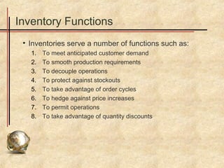
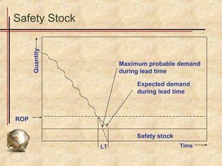
The document discusses inventory management concepts including: 1. Types of inventory like raw materials, work in process, and finished goods. 2. Inventory functions like meeting demand, smoothing production, and protecting against stockouts. 3. Effective inventory management requires tracking inventory levels, forecasting demand, and estimating costs of holding, ordering, and shortages. 4. Classification systems help prioritize inventory items for control based on factors like importance, value, or demand pattern.

1. Inventory Management
ABU BASHAR

2. Inventory
• Inventory
– A stock or store of goods
• Independent demand items
– Items that are ready to be sold or used

3. Types of Inventory
• Raw materials and purchased parts
• Work-in-process
• Finished goods inventories or merchandise
• Maintenance and repairs (MRO) inventory, tools and
supplies
• Goods-in-transit to warehouses or customers (pipeline
inventory)

4. Inventory Functions
• Inventories serve a number of functions such as:
1. To meet anticipated customer demand
2. To smooth production requirements
3. To decouple operations
4. To protect against stockouts
5. To take advantage of order cycles
6. To hedge against price increases
7. To permit operations
8. To take advantage of quantity discounts

5. Inventory Management
• Management has two basic functions
concerning inventory:
1. Establish a system for tracking items in inventory
2. Make decisions about
• When to order
• How much to order

6. Effective Inventory Management
• Requires:
1. A system keep track of inventory
2. A reliable forecast of demand
3. Knowledge of lead time and lead time variability
4. Reasonable estimates of
• holding costs
• ordering costs
• shortage costs
1. A classification system for inventory items

7. Inventory Counting Systems
• Periodic System
– Physical count of items in inventory made at
periodic intervals
• Perpetual Inventory System
– System that keeps track of removals from inventory
continuously, thus monitoring current levels of each
item
• Two-bin system
– Two containers of inventory; reorder
when the first is empty

8. Inventory Counting Technologies
• Universal product code (UPC)
– Bar code printed on a label that has information about
the item to which it is attached
• Radio frequency identification (RFID) tags
– A technology that uses radio waves to identify objects,
such as goods in supply chains

9. Demand Forecasts and Lead Time
• Forecasts
– Inventories are necessary to satisfy customer demands, so it is
important to have a reliable estimates of the amount and timing
of demand
• Lead time
– Time interval between ordering and receiving the order
• Point-of-sale (POS) systems
– A system that electronically records actual sales
– Such demand information is very useful for enhancing
forecasting and inventory management

10. ABC Classification System
• A-B-C approach
– Classifying inventory according to some measure of importance, and
allocating control efforts accordingly
– A items (very important)
• 10 to 20 percent of the number of items in inventory and about 60 to
70 percent of the annual dollar value
– B items (moderately important) High
– C items (least important)
• 50 to 60 percent of the number
of items in inventory but only Annual
A
$ value
about 10 to 15 percent of the of items
annual dollar value B
Low
C
Few Many
Number of Items

11. Cycle Counting
• Cycle counting
– A physical count of items in inventory
• Cycle counting management
– How much accuracy is needed?
• A items: ± 0.2 percent
• B items: ± 1 percent
• C items: ± 5 percent
– When should cycle counting be performed?
– Who should do it?

12. V-E-D Classification
• Based on the critical nature of items.
• Applicable to spare parts of equipment, as they
do not follow a predictable demand pattern.
• Very important in hospital pharmacy.

13. V-E-D Classification (Cont’d)
• V-Vital : Items without which the
activities will come to a halt.
• E-Essential : Items which are likely to
cause disruption of the
normal activity.
• D-Desirable : In the absence of which the
work does not get hampered.

14. H-M-L Classification
• Based on the unit value (in rupees) of items.
• Similar to A-B-C analysis
H-High
M-Medium
L -Low

15. F-S-N Classification
• Takes into account the distribution and handling
patterns of items from stores.
• Important when obsolescence is to be controlled.
F – Fast moving
S – Slow moving
N – Non moving

16. S-D-E Classification
• Based on the lead-time analysis and availability.
S – Scarce : longer lead time
D – Difficult : long lead time
E – Easy : reasonable lead time

17. S-O-S Classification
• S-O-S :Seasonal- Off- Seasonal
• Some items are seasonal in nature and hence
require special purchasing and stocking
strategies.
• EOQ formula cannot be applied in these cases.
• Inventories at the time of procurement will be
extremely high.

18. G-O-L-F Classification
• G-O-L-F stands for:
G – Government
O – Ordinary
L – Local
F – Foreign

19. X-Y-Z Classification
• Based on the value of inventory stored.
• If the values are high, special efforts should be
made to reduce them.
• This exercise can be done once a year.

20. Economic Order Quantity (EOQ):
Determining How Much to Order
• One of the oldest and most well known inventory
control techniques
• Easy to use
• Based on a number of assumptions

21. Assumptions of the EOQ Model
1. Demand is known and constant
2. Lead time is known and constant
3. Receipt of inventory is instantaneous
4. Quantity discounts are not available
5. Variable costs are limited to: ordering cost and
carrying (or holding) cost
6. If orders are placed at the right time, stock outs
can be avoided

22. Minimizing EOQ Model Costs
• Only ordering and carrying costs need to be
minimized (all other costs are assumed constant)
• As Q (order quantity) increases:
–Carry cost increases
–Ordering cost decreases (since the
number of orders per year decreases)

23. The Inventory Cycle
Profile of Inventory Level Over Time
Q Usage
Quantity rate
on hand
Reorder
point
Time
Receive Place Receive Place Receive
order order order order order
Lead time

24. EOQ Model Total Cost
At optimal order quantity (Q*):
Carrying cost = Ordering cost

25. Finding the Optimal Order Quantity
Parameters:
Q* = Optimal order quantity (the EOQ)
D = Annual demand
Co = Ordering cost per order
Ch = Carrying (or holding) cost per unit per yr
P = Purchase cost per unit

26. Two Methods for Carrying Cost
Carry cost (Ch) can be expressed either:
1. As a fixed cost, such as
Ch = $0.50 per unit per year
2. As a percentage of the item’s purchase cost
(P)
Ch = I x P
I = a percentage of the purchase cost

27. EOQ Total Cost
Total ordering cost = (D/Q) x Co
Total carrying cost = (Q/2) x Ch
Total purchase cost =PxD
= Total cost
Note:
• (Q/2) is the average inventory level
• Purchase cost does not depend on Q

28. Finding Q*
Recall that at the optimal order quantity (Q*):
Carry cost = Ordering cost
(D/Q*) x Co = (Q*/2) x Ch
Rearranging to solve for Q*:
Q* =
( 2 DCo / Ch )

29. EOQ Example: Sumco Pump Co.
Buys pump housing from a manufacturer and sells
to retailers
D = 1000 pumps annually
Co = $10 per order
Ch = $0.50 per pump per year
P = $5
Q* = ?

30. Example
• Zartex Co. produces fertilizer to sell to wholesalers. One
raw material – calcium nitrate – is purchased from a
nearby supplier at $22.50 per ton. Zartex estimates it will
need 5,750,000 tons of calcium nitrate next year.
• The annual carrying cost for this material is 40% of the
acquisition cost, and the ordering cost is $595.

31. Example
a) What is the most economical order quantity?
b) How many orders will be placed per year?

32. Example: Basic EOQ
• Economical Order Quantity (EOQ)
D = 5,750,000 tons/year
Ch = .40(22.50) = $9.00/ton/year
Co = $595/order
• Q* = ( 2 DCo / Ch )
EOQ = 2(5,750,000)(595)/9.00
= 27,573.135 tons per order

33. Example: Basic EOQ
• Total Annual Stocking Cost (TSC)
TSC = (Q/2)C + (D/Q)S
= (27,573.135/2)(9.00)
+ (5,750,000/27,573.135)(595)
= 124,079.11 + 124,079.11
= $248,158.22
Note: Total Carrying Cost
equals Total Ordering Cost

34. Example: Basic EOQ
• Number of Orders Per Year
= D/Q
= 5,750,000/27,573.135
= 208.5 orders/year

35. Economic Production Quantity (EPQ)
• Assumptions
– Only one product is involved
– Annual demand requirements are known
– Usage rate is constant
– Usage occurs continually, but production occurs periodically
– The production rate is constant
– Lead time does not vary
– There are no quantity discounts

36. EPQ
2 DS p
Q =
*
p
H p −u

37. When to Reorder
• Reorder point
– When the quantity on hand of an item drops to this amount, the
item is reordered.
– Determinants of the reorder point
1. The rate of demand
2. The lead time
3. The extent of demand and/or lead time variability
4. The degree of stockout risk acceptable to management

38. Reorder Point: Under Certainty
ROP = d × LT
where
d = Demand rate (units per period, per day, per week)
LT = Lead time (in same time units as d )

39. Reorder Point: Under Uncertainty
• Demand or lead time uncertainty creates the possibility
that demand will be greater than available supply
• To reduce the likelihood of a stockout, it becomes
necessary to carry safety stock
– Safety stock
• Stock that is held in excess of expected demand due to
variable demand and/or lead time
Expected demand
ROP = + Safety Stock
during lead time

40. Safety Stock
Quantity
Maximum probable demand
during lead time
Expected demand
during lead time
ROP
Safety stock
LT Time

41. Safety Stock?
• As the amount of safety stock carried increases, the risk
of stockout decreases.
– This improves customer service level
• Service level
– The probability that demand will not exceed supply during lead
time
– Service level = 100% - Stockout risk

42. How Much Safety Stock?
• The amount of safety stock that is appropriate
for a given situation depends upon:
1. The average demand rate and average lead time
2. Demand and lead time variability
3. The desired service level
Expected demand
ROP = + zσ dLT
during lead time
where
z = Number of standard deviations
σ dLT = The standard deviation of lead time demand

43. Reorder Point: Demand Uncertainty
ROP = d + zσ d LT
where
z = Number of standard deviations
d = Average demand per period (per day, per week)
σ d = The stddev. of demand per period (same time units as d )
LT = Lead time (same time units as d )

44. Reorder Point: Lead Time Uncertainty
ROP = d × LT + zdσ LT
where
z = Number of standard deviations
d = Demand per period (per day, per week)
σ LT = The stddev. of lead time (same time units as d )
LT = Average lead time (same time units as d )

45. How Much to Order: FOI
• Fixed-order-interval (FOI) model
– Orders are placed at fixed time intervals
• Reasons for using the FOI model
– Supplier’s policy may encourage its use
– Grouping orders from the same supplier can produce savings in
shipping costs
– Some circumstances do not lend themselves to continuously
monitoring inventory position

46. 120